Page 422 - Numerical Methods for Chemical Engineering

MCMC computation of posterior predictions 411

Example. Batch reactor chemical reaction data

We next use the MCMC approach to study again the hypothesis that the reaction
A + B → C is elementary, given the data in Table 8.1. We compute the 95% HPD
for the 2-D marginal posterior density p(θ 2 ,θ 3 |y). If this HPD region contains the
point (θ 2 = 1,θ 3 = 1), we cannot support the conclusion that the hypothesis is false
(i.e., the reaction is not elementary). We compute this marginal density using MCMC
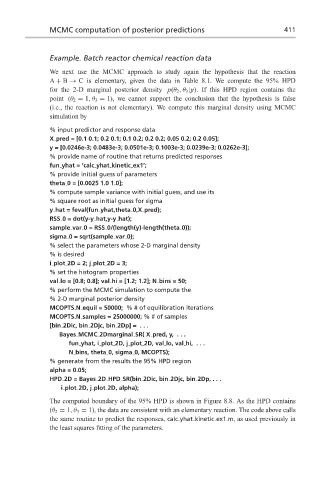
simulation by
% input predictor and response data
X pred = [0.1 0.1; 0.2 0.1; 0.1 0.2; 0.2 0.2; 0.05 0.2; 0.2 0.05];
y = [0.0246e-3; 0.0483e-3; 0.0501e-3; 0.1003e-3; 0.0239e-3; 0.0262e-3];
% provide name of routine that returns predicted responses
fun yhat = ‘calc yhat kinetic ex1’;
% provide initial guess of parameters
theta 0 = [0.0025 1.0 1.0];
% compute sample variance with initial guess, and use its
% square root as initial guess for sigma
y hat = feval(fun yhat,theta 0,X pred);
RSS 0 = dot(y-y hat,y-y hat);
sample var 0 = RSS 0/(length(y)-length(theta 0));
sigma 0 = sqrt(sample var 0);
% select the parameters whose 2-D marginal density
% is desired
i plot 2D=2;j plot 2D=3;
% set the histogram properties
val lo = [0.8; 0.8]; val hi = [1.2; 1.2]; N bins = 50;
% perform the MCMC simulation to compute the
% 2-D marginal posterior density
MCOPTS.N equil = 50000; % # of equilibration iterations
MCOPTS.N samples = 25000000; % # of samples
[bin 2Dic, bin 2Djc, bin 2Dp] = . . .
Bayes MCMC 2Dmarginal SR( X pred, y, . . .
fun yhat, i plot 2D, j plot 2D, val lo, val hi, . . .
N bins, theta 0, sigma 0, MCOPTS);
% generate from the results the 95% HPD region
alpha = 0.05;
HPD 2D = Bayes 2D HPD SR(bin 2Dic, bin 2Djc, bin 2Dp, . . .
i plot 2D, j plot 2D, alpha);
The computed boundary of the 95% HPD is shown in Figure 8.8. As the HPD contains
(θ 2 = 1,θ 3 = 1), the data are consistent with an elementary reaction. The code above calls
the same routine to predict the responses, calc yhat kinetic ex1.m, as used previously in
the least squares fitting of the parameters.