Page 426 - Numerical Methods for Chemical Engineering

Bayesian multiresponse regression 415

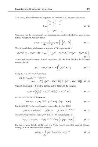
= cov(ε). From the measured responses, we form the N × L response data matrix
y
 [1] 
y [2]
 
  (8.180)
. 
.
Y = 
 . 
y [N]
We assume that the errors in each experiment are drawn independently from a multivariate
normal distribution with zero mean,

1 1 T −1
p(ε| ) = exp − ε ε (8.181)
(2π) L/2 | | 1/2 2
Thus, the probability of observing a response y [k] in experiment k is
1
[k] −L/2 −1/2 1 [k] [k] T −1 [k] [k]
p y |θ, = (2π) | | exp − y − f x ; θ y − f x ; θ
2
(8.182)
Assuming independent errors in each experiment, the likelihood function for the multi-
response data is
N
p y |θ,
l(θ, |Y) = p(Y|θ, ) = 0 [k] (8.183)
k=1
a b
Using the rule e e = e a+b ,wehave
l(θ, |Y) = (2π) −NL/2 | | −N/2
9 :
1 N [k] [k] T −1 [k] [k]
× exp − y − f x ; θ y − f x ; θ (8.184)
2 k=1
We next define the L × L positive-definite matrix S(θ) with the elements
N
[k]

[k]

S ab (θ) = y [k] − f a x ; θ y [k] − f b x ; θ (8.185)
a b
k=1
and write the likelihood function as
1

l(θ, |Y) = (2π) −NL/2 | | −N/2 exp − tr[ −1 S(θ)] (8.186)
2
For this l(θ, |Y), the noninformative prior is (Box & Tiao, 1973)
p(θ, ) = p(θ)p( ) p(θ) ∼ c p( ) ∝| | −(L+1)/2 (8.187)
Therefore, the posterior density p(θ, |Y) ∝ l(θ, |Y)p(θ)p( )is
1
1 −1
−(N+L+1)/2
−NL/2
p(θ, |Y) ∝ (2π) | | exp − tr[ S(θ)] (8.188)
2
For this posterior density, of the form of a Wishart distribution, the marginal posterior
density for θ can be computed analytically:
'
−N/2
p(θ|Y) = p(θ, |Y)d ∝ |S(θ)| (8.189)
>0