Page 421 - Numerical Methods for Chemical Engineering

410 8 Bayesian statistics and parameter estimation

2

1

1
θ 2

−

1 1 11 11 12 12
θ 1

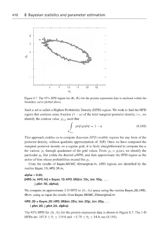
Figure 8.7 The 95% HPD region for (θ 1 , θ 2 ) for the protein expression data is enclosed within the
boundary curve plotted above.

Such a set is called a Highest Probability Density (HPD) region. We wish to find the HPD
region that contains some fraction (1 − α) of the total marginal posterior density; i.e., we
identify the contour value p c,α such that
'
p(ψ|y)dψ = 1 − α (8.168)
p c,α
This approach enables us to compute Bayesian HPD credible regions for any form of the
posterior density, without quadratic approximation of S(θ). Once we have computed the
marginal posterior density on a regular grid, it is fairly straightforward to compute the α
for various p c through quadrature of the grid values. From p c = p c (α), we identify the
particular p c that yields the desired αHPD, and then approximate the HPD region as the
union of bins whose probabilities exceed this p c .
From the results of Bayes MCMC 1Dmarginal.m, HPD regions are identified by the
routine Bayes 1D HPD SR.m,

alpha = 0.05;
[HPD lo, HPD hi] = Bayes 1D HPD SR(bin 1Dc, bin 1Dp, . . .
j plot 1D, alpha);
We compute an approximate 2-D HPD in (θ 1 ,θ 2 ) space using the routine Bayes 2D HPD
SR.m, using as input the results from Bayes MCMC 2Dmarginal.m:

HPD 2D = Bayes 2D HPD SR(bin 2Dic, bin 2Djc, bin 2Dp,...
i plot 2D, j plot 2D, alpha);

The 95% HPD for (θ 1 ,θ 2 ) for the protein expression data is shown in Figure 8.7. The 1-D
HPDs are 107.8 ≤ θ 1 ≤ 119.0 and −1.78 ≤ θ 2 ≤ 14.0, see (8.145).