Page 424 - Numerical Methods for Chemical Engineering

Applying eigenvalue analysis to experimental design 413

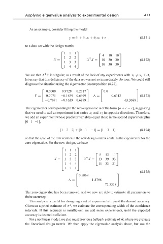
As an example, consider fitting the model

y = θ 1 + θ 2 x 1 + θ 3 x 2 + ε (8.171)

to a data set with the design matrix
111  
 
4 10 10
122
  T
X =   X X =  10 30 30  (8.172)
 133 
10 30 30
144
T
We see that X X is singular, as a result of the lack of any experiments with x 1 = x 2 . But,
let us say that this deficiency of the data set was not so immediately obvious. We could still
diagnose the situation using the eigenvector decomposition (8.27),
   
0.0000 0.9728 0.2317 0.0
V =  0.7071 −0.1639 0.6979  =  0.6312  (8.173)
−0.7071 −0.1639 0.6879 63.3688

The eigenvector corresponding to the zero eigenvalue is of the form [o + c − c], suggesting
that we need to add an experiment that varies x 1 and x 2 in opposite directions. Therefore,
we add an experiment whose predictor variables equal those in the second experiment plus
[0 1 −1],

[122] + [01 −1] = [131] (8.174)

so that the span of the row vectors in the new design matrix contains the eigenvector for the
zero eigenvalue. For the new design, we have
 
111
5 13 11
 
 
 122 
T
 
X X =  13 39 33 
X =  133 
11 33 31
 
 144 
131
(8.175)
 
0.5868
=  1.8796 
72.5338
The zero eigenvalue has been removed, and we now are able to estimate all parameters to
finite accuracy.
This analysis is useful for designing a set of experiments to yield the desired accuracy.
2
Given an a priori estimate of σ , we estimate the corresponding width of the confidence
intervals. If this accuracy is insufficient, we add more experiments, until the expected
accuracy is deemed sufficient.
For a nonlinear model, we also must provide a ballpark estimate of θ, where we evaluate
the linearized design matrix. We then apply the eigenvalue analysis above, but use the