Page 427 - Numerical Methods for Chemical Engineering

416 8 Bayesian statistics and parameter estimation

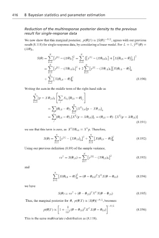
Reduction of the multiresponse posterior density to the previous
result for single-response data
−N/2
We now show that this marginal posterior, p(θ|Y) ∝|S(θ)| , agrees with our previous
[k]
result (8.118) for single-response data, by considering a linear model. For L = 1, ˆ y (θ) =
(Xθ) k ,
N N

S(θ) = y [k] − (Xθ) k 2 = y [k] − (Xθ LS ) k + X θ LS − θ 2
k
k=1 k=1
N N

= y [k] − (Xθ LS ) k 2 + 2 y [k] − (Xθ LS ) k X(θ LS − θ)
k
k=1 k=1
N
2

+ X(θ LS − θ) (8.190)
k
k=1
Writing the sum in the middle term of the right-hand side as

N

X kj θ LS − θ
(y − X θ LS ) k
j
k=1 j
N
T

= (θ LS − θ) j (X ) jk y − Xθ LS
k
j k=1
T T
= (θ LS − θ) j [X (y − Xθ LS )] j = (θ LS − θ) · [X (y − Xθ LS )]
j
(8.191)
T
T
we see that this term is zero, as X Xθ LS = X y. Therefore,
N N

S(θ) = y [k] − Xθ LS 2 + X(θ LS − θ) 2 (8.192)
k k
k=1 k=1
Using our previous definition (8.89) of the sample variance,
N
2 [k] 2
νs = S(θ LS ) = y − (Xθ LS ) k (8.193)
k=1
and
N
2

T T
X(θ LS − θ) = (θ − θ LS ) X X(θ − θ LS ) (8.194)
k
k=1
we have
T
T
2
S(θ) = νs + (θ − θ LS ) X X(θ − θ LS ) (8.195)
−N/2
Thus, the marginal posterior for θ, p(θ|Y) ∝|S(θ)| , becomes
1 T T
−N/2
p(θ|Y) ∝ 1 + (θ − θ LS ) X X(θ − θ LS ) (8.196)
νs 2
This is the same multivariate t-distribution as (8.118).