Page 423 - Numerical Methods for Chemical Engineering

412 8 Bayesian statistics and parameter estimation

11

11

1

θ 1

1 1 11 11
θ 2
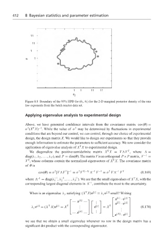
Figure 8.8 Boundary of the 95% HPD for (θ 2 ,θ 3 ) for the 2-D marginal posterior density of the rate
law exponents from the batch reactor data set.

Applying eigenvalue analysis to experimental design

Above, we have generated confidence intervals from the covariance matrix cov(θ) =
−1
T
2
2
σ (X X) . While the value of σ may be determined by fluctuations in experimental
conditions that are beyond our control, we can control, through our choice of experimental
design, the design matrix X. We would like to design our experiments so that they provide
enough information to estimate the parameters to sufficient accuracy. We now consider the
T
application of eigenvalue analysis of X X to experimental design.
T T
We diagonalize the positive-semidefinite matrix X X = V V , where =
diag(λ 1 ,λ 2 ,...,λ P ),and P = dim(θ).ThematrixVisanorthogonal P×P matrix, V −1 =
T
T
V , whose columns contain the normalized eigenvectors of X X. The covariance matrix
of θ is
T −1
2
2
−1
2
−1
cov(θ) = σ [V V ] = σ V T(−1) V −1 = σ V V T (8.169)
−1
T
−1
−1
where −1 = diag(λ ,λ ,...,λ ). We see that the small eigenvalues of X X, with the
1 2 P
−1
corresponding largest diagonal elements in , contribute the most to the uncertainty.
T
When is an eigenvalue λ j satisfying (X X)v [ j] = λ j v [ j] small? Writing
 [1] [ j] 
 [1]  x · v
— x —  
|  x [2] · v [ j] 
T
v
λ j v [ j] = (X X)v [ j] T  . .   [ j]  T  .  (8.170)
.  = X  . 
= X 
 . 
— x [N] — | [N] [ j]
x · v
we see that we obtain a small eigenvalue whenever no row in the design matrix has a
significant dot product with the corresponding eigenvector.