Page 418 - Numerical Methods for Chemical Engineering

MCMC computation of posterior predictions 407

and
% calc g 1Dinterval.m
function g = calc g 1Dinterval(theta,sigma,Param);
if((theta(Param.j) >= Param.val lo) & . . .
(theta(Param.j) <= Param.val hi))
g=1;
else
g=0;
end
return;

The output from this program is
g pred = 0.7233

Thus, we compute a ∼72.3% chance that the mutant strain has a protein expression level
that is greater than or equal to five units above that of the wild-type strain.

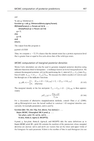
MCMC computation of marginal posterior densities

Monte Carlo simulation can also be used to generate marginal posterior densities using
indicator functions fitted to histograms – a technique known as kernel marginalization.We
estimate the marginal posterior p(θ j |y) by partitioning the θ j interval [θ j,lo ,θ j,hi ] into N bins
bins of width j,bin = (θ j,hi − θ j,lo )/N bins . We measure the relative number of visits to each
bin through use of the indicator functions

1, [θ j,lo + (k − 1) j,bin ] ≤ θ j < [θ j,lo + k j,bin ]
g j,k (θ,σ) = (8.165)
0, otherwise
1
The marginal density at the bin mid-point θ j,k = θ j,lo + (k − ) j,bin is then approxi-
2
mately
E[g j,k |y]
p(θ j,k |y) ≈ (8.166)
j,bin
For a discussion of alternative marginalization methods, consult Chen et al. (2000).
calc g 1Dmarginal.m uses the kernel method to construct 1-D marginal densities con-
currently for multiple parameters, and is used by

function [bin 1Dc, bin 1Dp, frac above, frac below] = . . .
Bayes MCMC 1Dmarginal SR( X pred, y, . . .
fun yhat, j plot 1D, val lo, val hi, . . .
N bins, theta 0, sigma 0, MCOPTS);

X pred, y, fun yhat, theta 0, sigma 0, and MCOPTS take the same definitions as in
Bayes MCMC pred SR. j plot 1D contains the numbers of the parameters whose marginal
densities are desired. val lo and val hi are vectors that set the lower and upper limits of
the histogram for each parameter. N bins is the number of bins in each histogram (we use