Page 420 - Numerical Methods for Chemical Engineering

MCMC computation of posterior predictions 409

2
1

1 2
1
12 1
θ 2 1
1

2

1 1 11 11 12
θ 1
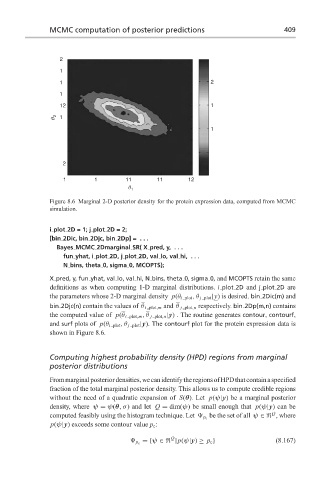
Figure 8.6 Marginal 2-D posterior density for the protein expression data, computed from MCMC
simulation.

i plot 2D=1;j plot 2D=2;
[bin 2Dic, bin 2Djc, bin 2Dp] = . . .
Bayes MCMC 2Dmarginal SR( X pred, y, . . .
fun yhat, i plot 2D, j plot 2D, val lo, val hi, . . .
N bins, theta 0, sigma 0, MCOPTS);
X pred, y, fun yhat, val lo, val hi, N bins, theta 0, sigma 0, and MCOPTS retain the same
definitions as when computing 1-D marginal distributions. i plot 2D and j plot 2D are
the parameters whose 2-D marginal density p(θ i plot ,θ j plot |y) is desired. bin 2Dic(m) and
bin 2Djc(n) contain the values of θ i plot,m and θ j plot,n respectively. bin 2Dp(m,n) contains
the computed value of p(θ i plot,m , θ j plot,n |y) . The routine generates contour, contourf,
and surf plots of p(θ i plot ,θ j plot |y). The contourf plot for the protein expression data is
shown in Figure 8.6.

Computing highest probability density (HPD) regions from marginal
posterior distributions

Frommarginalposteriordensities,wecanidentifytheregionsofHPDthatcontainaspecified
fraction of the total marginal posterior density. This allows us to compute credible regions
without the need of a quadratic expansion of S(θ). Let p(ψ|y) be a marginal posterior
density, where ψ = ψ(θ,σ) and let Q = dim(ψ) be small enough that p(ψ|y) can be
Q
be the set of all ψ ∈ , where
computed feasibly using the histogram technique. Let p c
p(ψ|y) exceeds some contour value p c :
Q
={ψ ∈ |p(ψ|y) ≥ p c } (8.167)
p c