Page 429 - Numerical Methods for Chemical Engineering

418 8 Bayesian statistics and parameter estimation

Use of this routine requires the MATLAB optimization toolkit, for access to fminsearch,
when freq quench is nonzero. If fminsearch is unavailable, the routine may be modified
to use the conjugate gradient minimizer routine provided in Chapter 5.

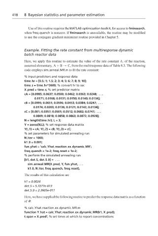
Example. Fitting the rate constant from multiresponse dynamic
batch reactor data
Here, we apply this routine to estimate the value of the rate constant k 1 of the reaction,
assumed elementary, A + B → C, from the multiresponse data of Table 8.3. The following
code employs sim anneal MR.m to fit the rate constant:

% input predictors and response data
time hr = [0.5; 1; 1.5; 2; 3; 4; 5; 6; 7; 8; 9; 10];
time s = time hr*3600; % convert hr to sec
X pred = time s; % set predictor matrix
cA = [0.0985; 0.0637; 0.0500; 0.0462; 0.0363; 0.0248; . . .
0.0171; 0.0168; 0.0131; 0.0150; 0.0140; 0.0134];
cB = [0.0995; 0.0651; 0.0596; 0.0453; 0.0384; 0.0247; . . .
0.0174; 0.0203; 0.0136; 0.0121; 0.0142; 0.0134];
cC = [0.001; 0.0357; 0.0501; 0.0512; 0.0682; 0.0747; . . .
0.0809; 0.0818; 0.0858; 0.0863; 0.0872; 0.0928];
N = length(time hr);L=3;
Y = zeros(N,L); % set response data matrix
Y(:,1) = cA; Y(:,2) = cB; Y(:,3) = cC;
% set parameters for simulated annealing run
N iter = 1000;
k1 0 = 0.001;
fun yhat = ‘calc Yhat reaction ex dynamic MR’;
freq quench = 1e-2; freq reset = 1e-2;
% perform the simulated annealing run
[k1, det S, det S 0] = ...
sim anneal MR(X pred, Y, fun yhat, . . .
k1 0, N iter, freq quench, freq reset),
The results of this calculation are

k1 = 0.0024
det S = 5.7277e-013
det S 0 = 2.3605e-011
Here, we have supplied the following routine to predict the response data matrix as a function
of θ:
% calc Yhat reaction ex dynamic MR.m
function Y hat = calc Yhat reaction ex dynamic MR(k1, X pred);
t span = X pred’; % set times at which to report concentrations