Page 433 - Numerical Methods for Chemical Engineering

422 8 Bayesian statistics and parameter estimation

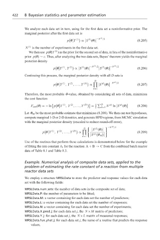
We analyze each data set in turn, using for the first data set a noninformative prior. The
marginal posterior after the first data set is
−N 1 /2

1
p θ Y 1 ∝ S (θ) (8.205)

N 1 is the number of experiments in the first data set.
We then use p(θ|Y 1 ) as the prior for the second set of data, in lieu of the noninformative
prior p(θ) ∼ c. Thus, after analyzing the two data sets, Bayes’ theorem yields the marginal
posterior density
/2
−N 1 −N 2 /2
S (θ)
1
p θ Y 1 , Y 2 ∝ S (θ) 2 (8.206)

Continuing this process, the marginal posterior density with all D sets is
D
0 −N d /2
p θ Y 1 , Y 2 ,..., Y D ∝ d (θ) (8.207)
S

d=1
Therefore, the most probable θ-value, obtained by considering all sets of data, minimizes
the cost function
1 D
d
F cost (θ) =− ln p θ Y 1 , Y 2 ,..., Y D = N d ln S (θ) (8.208)

2 d=1
Let θ M be the most probable estimate that minimizes (8.208). We then can test hypotheses,
compute marginal 1-D or 2-D densities, and generate HPD regions, from MCMC simulation
with the marginal posterior density (rescaled to reduce round-off error),
−N d /2
D d
(
0 S (θ)

p θ Y 1 , Y 2 ,..., Y D ∝ (8.209)

S
d
d=1 θ M
Use of the routines that perform these calculations is demonstrated below for the example
of fitting the rate constant k 1 for the reaction A + B → C from the combined batch reactor
data of Table 8.1 and Table 8.3.
Example. Numerical analysis of composite data sets, applied to the
problem of estimating the rate constant of a reaction from multiple
reactor data sets
We employ a structure MRSLData to store the predictor and response values for each data
set with the following fields:
MRSLData.num sets: the number of data sets in the composite set of data;
MRSLData.P: the number of parameters to be fitted;
MRSLData.M: a vector containing for each data set the number of predictors;
MRSLData.L: a vector containing for each data set the number of responses;
MRSLData.N: a vector containing for each data set the number of experiments;
MRSLData.X pred j: for each data set j, the N ×M matrix of predictors;
MRSLData.Y j: for each data set j, the N ×L matrix of measured responses;
MRSLData.fun yhat j: for each data set j, the name of a routine that predicts the response
values,