Page 437 - Numerical Methods for Chemical Engineering

426 8 Bayesian statistics and parameter estimation

×1
2

2

1
)

(θ 1
1

2 22 2 2 2
−
θ 1 ×1
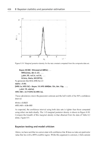
Figure 8.10 Marginal posterior density for the rate constant computed from the composite data set.

Bayes MCMC 1Dmarginal MRSL(...
MRSLData, det S ref, . . .
j plot 1D, val lo, val hi, . . .
N bins, theta, MCOPTS);
% generate the 95% HPD for k1
alpha = 0.05;
[HPD lo, HPD hi] = Bayes 1D HPD MR(bin 1Dc, bin 1Dp, . . .
j plot 1D, alpha);
HPD HW = 0.5*(HPD hi-HPD lo),
These calculations return the parameter estimate and the half-width of the 96% confidence
interval:

theta = 0.0025
HPD HW = 4.8e-005

As expected, the confidence interval using both data sets is tighter than those computed
using either one individually. The 1-D marginal posterior density is shown in Figure 8.10.
Compare the breadth of this marginal density to that obtained from the data of Table 8.3
alone, Figure 8.9.

Bayesian testing and model criticism

Above, we have said that we cannot state with confidence that θ does not take any particular
value that lies with a HPD credible region. While this argument is common, it falls outside