Page 436 - Numerical Methods for Chemical Engineering

Analysis of composite data sets 425

The arguments N iter, freq quench, freq reset, and T 0 have the same definitions as pre-
[0]
viously. If T 0 is not included in the list of arguments, a default value of 10|F cost (θ )| is
used.
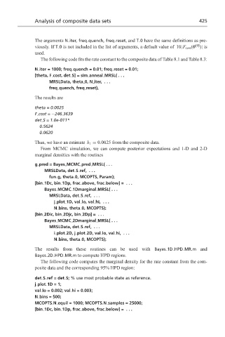
The following code fits the rate constant to the composite data of Table 8.1 and Table 8.3:

N iter = 1000; freq quench = 0.01; freq reset = 0.01;
[theta, F cost, det S] = sim anneal MRSL( . . .
MRSLData, theta 0, N iter, . . .
freq quench, freq reset),

The results are
theta = 0.0025
F cost = −246.3639
det S = 1.0e-011*
0.5624
0.0620
Thus, we have an estimate k 1 = 0.0025 from the composite data.
From MCMC simulation, we can compute posterior expectations and 1-D and 2-D
marginal densities with the routines
g pred = Bayes MCMC pred MRSL( . . .
MRSLData, det S ref, . . .
fun g, theta 0, MCOPTS, Param);
[bin 1Dc, bin 1Dp, frac above, frac below] = . . .
Bayes MCMC 1Dmarginal MRSL( . . .
MRSLData, det S ref, . . .
j plot 1D, val lo, val hi, . . .
N bins, theta 0, MCOPTS);
[bin 2Dic, bin 2Djc, bin 2Dp] = . . .
Bayes MCMC 2Dmarginal MRSL( . . .
MRSLData, det S ref, . . .
i plot 2D, j plot 2D, val lo, val hi, . . .
N bins, theta 0, MCOPTS);
The results from these routines can be used with Bayes 1D HPD MR.m and
Bayes 2D HPD MR.m to compute HPD regions.
The following code computes the marginal density for the rate constant from the com-
posite data and the corresponding 95% HPD region:

det S ref = det S; % use most probable state as reference.
j plot 1D=1;
val lo = 0.002; val hi = 0.003;
N bins = 500;
MCOPTS.N equil = 1000; MCOPTS.N samples = 25000;
[bin 1Dc, bin 1Dp, frac above, frac below] = . . .