Page 440 - Numerical Methods for Chemical Engineering

Bayesian testing and model criticism 429

N
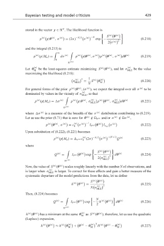
stored in the vector y ∈ . The likelihood function is
(

S α θ α
−N/2 α −N

p α y|θ α ,σ α = (2π) σ (8.218)
2
exp −
2 σ α
and the integral (8.215) is
' '
∞

p α (y|M α ) = dσ α p α y|θ α ,σ α p α θ α ,σ α dθ α (8.219)
0
P α

α
Let θ α be the least-squares estimate minimizing S α (θ α ), and let σ MLE be the value
M
maximizing the likelihood (8.218):
2 1
α α
σ = S α θ (8.220)
MLE M
N
For general forms of the prior p α (θ α , (σ α ), we expect the integral over all σ α to be
dominated by values in the vicinity of σ α , so that
MLE
'
α α
p α (y|M α ) = σ α p α y|θ α ,σ p α θ α ,σ dθ α (8.221)
MLE MLE
P α
where σ α is a measure of the breadth of the σ α distribution contributing to (8.219).
Let us use the prior (8.71) that is zero for θ α / ∈ θ α and/or σ α / ∈ σ α ,

α α −1
p α θ α ,σ α = c σ α θ α σ α (8.222)
0 I θ I σ α
Upon substitution of (8.222), (8.221) becomes

p α (y|M α ) = σ c α (2π) −N/2 σ α −(N+1) Q α (8.223)
α
0
where
(

S θ
' α α

Q α = I θ α θ α exp − 2 dθ α (8.224)
α
2 σ MLE
P α

Now, the value of S α (θ α ) scales roughly linearly with the number N of observations, and
is larger when σ α is larger. To correct for these effects and gain a better measure of the
MLE
systematic departure of the model predictions from the data, let us define

S α θ α

h α θ α = (8.225)
α 2
N σ
MLE
Then, (8.224) becomes
N
' 1

Q α = I θ α θ α exp − h α θ α dθ α (8.226)
2
P α

h α (θ α ) has a minimum at the same θ α as S α (θ α ); therefore, let us use the quadratic
M
(Laplace) expansion,
α α T α

h α θ α ≈ h α θ + θ α − θ H α θ α − θ (8.227)
M M M