Page 443 - Numerical Methods for Chemical Engineering

432 8 Bayesian statistics and parameter estimation

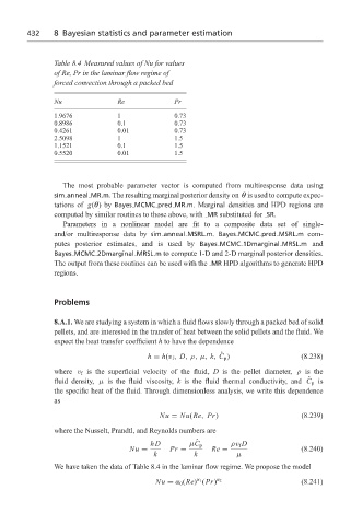
Table 8.4 Measured values of Nu for values
of Re, Pr in the laminar flow regime of
forced convection through a packed bed

Nu Re Pr

1.9676 1 0.73
0.8986 0.1 0.73
0.4261 0.01 0.73
2.5098 1 1.5
1.1521 0.1 1.5
0.5520 0.01 1.5

The most probable parameter vector is computed from multiresponse data using
sim anneal MR.m. The resulting marginal posterior density on θ is used to compute expec-
tations of g(θ)by Bayes MCMC pred MR.m. Marginal densities and HPD regions are
computed by similar routines to those above, with MR substituted for SR.
Parameters in a nonlinear model are fit to a composite data set of single-
and/or multiresponse data by sim anneal MSRL.m. Bayes MCMC pred MSRL.m com-
putes posterior estimates, and is used by Bayes MCMC 1Dmarginal MRSL.m and
Bayes MCMC 2Dmarginal MRSL.m to compute 1-D and 2-D marginal posterior densities.
The output from these routines can be used with the MR HPD algorithms to generate HPD
regions.

Problems

8.A.1. We are studying a system in which a fluid flows slowly through a packed bed of solid
pellets, and are interested in the transfer of heat between the solid pellets and the fluid. We
expect the heat transfer coefficient h to have the dependence
ˆ
h = h(v f , D,ρ,µ, k, C p ) (8.238)
where v f is the superficial velocity of the fluid, D is the pellet diameter, ρ is the
ˆ
fluid density, µ is the fluid viscosity, k is the fluid thermal conductivity, and C p is
the specific heat of the fluid. Through dimensionless analysis, we write this dependence
as

Nu = Nu(Re, Pr) (8.239)
where the Nusselt, Prandtl, and Reynolds numbers are
ˆ
hD µC p ρv f D
Nu = Pr = Re = (8.240)
k k µ
We have taken the data of Table 8.4 in the laminar flow regime. We propose the model

Nu = α 0 (Re) (Pr) α 2 (8.241)
α 1