Page 438 - Numerical Methods for Chemical Engineering

Bayesian testing and model criticism 427

of the structure of statistical decision theory. We present here the Bayesian approach to
evaluating the relative merits of alternative hypotheses or models, Bayesian testing.

Null hypothesis testing

We begin by considering, after taking the data Y, which of two hypotheses is more probably
P
true. Let the null hypothesis H 0 be that θ ∈ 0 ⊂ , and let the alternative hypothesis H 1
P
be that θ ∈ 1 ⊂ . Often, 1 is the complement set to 0 so that H 1 is the hypothesis
that θ /∈ 0 . The prior and posterior probabilities of each hypothesis being true are

' '
P(H j ) = p(θ)dθ P(H j |Y) = p(θ|Y)dθ (8.210)
j j

where the marginalized priors and posteriors are p(θ) and p(θ|Y) respectively. For P(H j )
to be defined, we again require p(θ) to be proper. We would like to control, in some sense,
the effect of the prior to see what the data are telling us about which hypothesis is more
likely to be true. Therefore, to compare the relative amounts by which the data increase or
decrease our beliefs in the hypotheses, we compute the Bayes factor

P(H 0 |Y)/P(H 0 )
B 01 (Y) = (8.211)
P(H 1 |Y)/P(H 1 )

If B 01 (Y) 1, H 0 is favored by the data. If B 01 (Y) 1, H 1 is favored. The exact value of
B 01 (Y) is quite sensitive to the choice of prior, and in particular, we cannot use improper
priors here. Let us say that we have used the simple fix (8.71) of setting p(θ) to zero outside
of θ and to a uniform value inside θ . Then, P(H j ) is merely the ratio of the volume
of j to that of θ , and is thus highly sensitive to the (subjective) choice of θ . For an
improper prior with j of finite volume, P(H j ) is zero and the Bayes factor is not defined.
Robert (2001) discusses alternative means to make proper a prior using training sets to fit
a prior and then applying Bayesian analysis to the remaining data; however, such methods
fall somewhat outside of the Bayesian paradigm. For now, we retain the use of (8.71), yet
note that the boundaries of θ should be selected with some care. Clearly, we should attach
significance to the value of the Bayes factor only if it is far greater or far less than 1. Jeffreys
(1961) suggests the following interpretation:

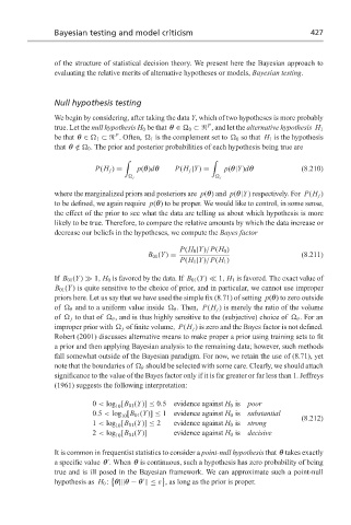
0 < log [B 01 (Y)] ≤ 0.5 evidence against H 0 is poor
10
0.5 < log [B 01 (Y)] ≤ 1 evidence against H 0 is substantial
10 (8.212)
1 < log [B 01 (Y)] ≤ 2 evidence against H 0 is strong
10
2 < log [B 01 (Y)] evidence against H 0 is decisive
10
It is common in frequentist statistics to consider a point-null hypothesis that θ takes exactly
a specific value θ . When θ is continuous, such a hypothesis has zero probability of being

true and is ill posed in the Bayesian framework. We can approximate such a point-null

hypothesis as H 0 : θ| θ − θ ≤ ε , as long as the prior is proper.