Page 434 - Numerical Methods for Chemical Engineering

Analysis of composite data sets 423

Y hat = feval(fun yhat j, theta, X pred j);
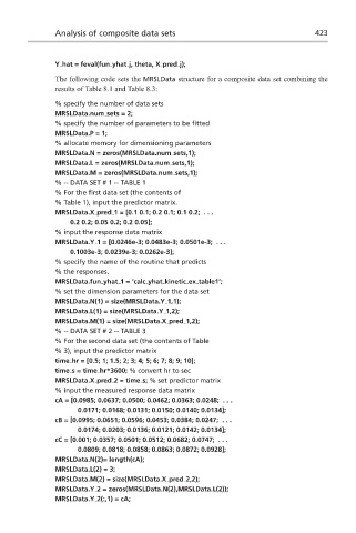
The following code sets the MRSLData structure for a composite data set combining the
results of Table 8.1 and Table 8.3:
% specify the number of data sets
MRSLData.num sets = 2;
% specify the number of parameters to be fitted
MRSLData.P = 1;
% allocate memory for dimensioning parameters
MRSLData.N = zeros(MRSLData.num sets,1);
MRSLData.L = zeros(MRSLData.num sets,1);
MRSLData.M = zeros(MRSLData.num sets,1);
%--DATASET#1--TABLE 1
% For the first data set (the contents of
% Table 1), input the predictor matrix.
MRSLData.X pred 1 = [0.1 0.1; 0.2 0.1; 0.1 0.2; . . .
0.2 0.2; 0.05 0.2; 0.2 0.05];
% input the response data matrix
MRSLData.Y 1 = [0.0246e-3; 0.0483e-3; 0.0501e-3; . . .
0.1003e-3; 0.0239e-3; 0.0262e-3];
% specify the name of the routine that predicts
% the responses.
MRSLData.fun yhat 1 = ‘calc yhat kinetic ex table1’;
% set the dimension parameters for the data set
MRSLData.N(1) = size(MRSLData.Y 1,1);
MRSLData.L(1) = size(MRSLData.Y 1,2);
MRSLData.M(1) = size(MRSLData.X pred 1,2);
%--DATASET#2--TABLE 3
% For the second data set (the contents of Table
% 3), input the predictor matrix
time hr = [0.5; 1; 1.5; 2; 3; 4; 5; 6; 7; 8; 9; 10];
time s = time hr*3600; % convert hr to sec
MRSLData.X pred 2 = time s; % set predictor matrix
% input the measured response data matrix
cA = [0.0985; 0.0637; 0.0500; 0.0462; 0.0363; 0.0248; . . .
0.0171; 0.0168; 0.0131; 0.0150; 0.0140; 0.0134];
cB = [0.0995; 0.0651; 0.0596; 0.0453; 0.0384; 0.0247; . . .
0.0174; 0.0203; 0.0136; 0.0121; 0.0142; 0.0134];
cC = [0.001; 0.0357; 0.0501; 0.0512; 0.0682; 0.0747; . . .
0.0809; 0.0818; 0.0858; 0.0863; 0.0872; 0.0928];
MRSLData.N(2)= length(cA);
MRSLData.L(2) = 3;
MRSLData.M(2) = size(MRSLData.X pred 2,2);
MRSLData.Y 2 = zeros(MRSLData.N(2),MRSLData.L(2));
MRSLData.Y 2(:,1) = cA;