Page 448 - Numerical Methods for Chemical Engineering

Fourier series and transforms in one dimension 437

˜
Next, we compute a n , n = 1, 2, 3,...by multiplying both f (t) and f (t) by cos(nπt/P)
and integrating over [0, 2P]:
2P 2P
nπt nπt

' '
f (t) cos dt = ˜ f (t) cos dt (9.5)
P P
0 0
Using the orthogonality properties
2 P 2P

mπt nπt mπt nπt
' '
cos cos dt = sin sin dt = Pδ mn
P P P P
0 0 (9.6)
2P

mπt nπt
'
sin cos dt = 0
P P
0
we obtain
2P

1 nπt
'
a n = f (t) cos dt n = 1, 2, 3,... (9.7)
P P
0
A similar procedure, but multiplying by sin(nπt/P) instead, yields
2P
1 ' nπt
b n = f (t) sin dt n = 1, 2, 3,... (9.8)
P P
0
The summations above are over an infinite number of terms, but if we truncate the series to
some finite order N, we obtain an approximate Fourier representation of the function:
N
1 mπt mπt
f (t) ≈ a 0 + a m cos + b m sin (9.9)
2 P P
m=1
To compute the 2N + 1 coefficients of this expansion, we might consider using numerical
quadrature for the necessary integrals; however, as N increases, so does the required number
of quadrature points, as the sine and cosine basis functions vary more rapidly with increasing
m. Thus, the amount of work necessary to obtain an approximate Fourier representation in
2
this manner scales as N . Below, we consider an alternative method that requires only
2
N log N « N operations.
2
Gibbs oscillations
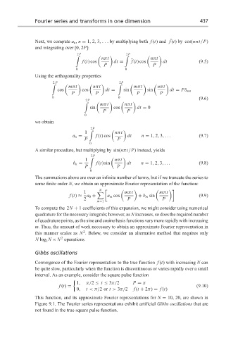
Convergence of the Fourier representation to the true function f (t) with increasing N can
be quite slow, particularly when the function is discontinuous or varies rapidly over a small
interval. As an example, consider the square pulse function

1, π/2 ≤ t ≤ 3π/2 P = π
f (t) = (9.10)
0, t <π/2or t > 3π/2 f (t + 2π) = f (t)
This function, and its approximate Fourier representations for N = 10, 20, are shown in
Figure 9.1. The Fourier series representations exhibit artificial Gibbs oscillations that are
not found in the true square pulse function.