Page 449 - Numerical Methods for Chemical Engineering

438 9 Fourier analysis

a 1
t
t
1 ar
t
ar
t

1 2
t
1
t
t
1 ar
t
ar
t

1 2
t
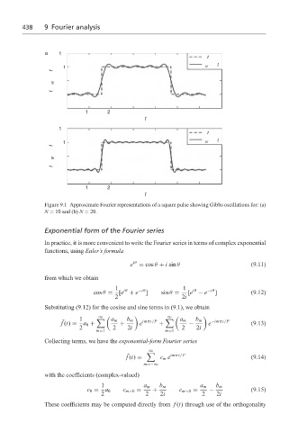
Figure 9.1 Approximate Fourier representations of a square pulse showing Gibbs oscillations for: (a)
N = 10 and (b) N = 20.

Exponential form of the Fourier series

In practice, it is more convenient to write the Fourier series in terms of complex exponential
functions, using Euler’s formula

iθ
e = cos θ + i sin θ (9.11)
from which we obtain
1 iθ −iθ 1 iθ −iθ
cos θ = [e + e ] sin θ = [e − e ] (9.12)
2 2i
Substituting (9.12) for the cosine and sine terms in (9.1), we obtain
∞
∞
1 a m b m a m b m
˜ imπt/P −imπt/P
f (t) = a 0 + + e + − e (9.13)
2 2 2i 2 2i
m=1 m=1
Collecting terms, we have the exponential-form Fourier series
∞

˜ imπt/P
f (t) = c m e (9.14)
m=−∞
with the coefficients (complex-valued)
1 a m b m a m b m
c 0 = a 0 c m>0 = + c m<0 = − (9.15)
2 2 2i 2 2i
These coefficients may be computed directly from f (t) through use of the orthogonality