Page 47 - Numerical Methods for Chemical Engineering

36 1 Linear algebra

A
ℜ ℜ
1
x A b
b Ax
A 1

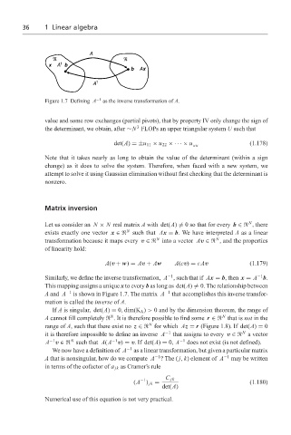
Figure 1.7 Defining A −1 as the inverse transformation of A.

value and some row exchanges (partial pivots), that by property IV only change the sign of
3
the determinant, we obtain, after ∼N FLOPs an upper triangular system U such that
det(A) =±u 11 × u 22 × ··· × u (1.178)
NN
Note that it takes nearly as long to obtain the value of the determinant (within a sign
change) as it does to solve the system. Therefore, when faced with a new system, we
attempt to solve it using Gaussian elimination without first checking that the determinant is
nonzero.

Matrix inversion

N
Let us consider an N × N real matrix A with det(A) = 0 so that for every b ∈ , there
N
exists exactly one vector x ∈ such that Ax = b. We have interpreted A as a linear
N
N
transformation because it maps every v ∈ into a vector Av ∈ , and the properties
of linearity hold:
A(v + w) = Av + Aw A(cv) = cAv (1.179)

−1
−1
Similarly, we define the inverse transformation, A , such that if Ax = b, then x = A b.
This mapping assigns a unique x to every b as long as det(A) = 0. The relationship between
A and A −1 is shown in Figure 1.7. The matrix A −1 that accomplishes this inverse transfor-
mation is called the inverse of A.
If A is singular, det(A) = 0, dim(K A ) > 0 and by the dimension theorem, the range of
N
N
A cannot fill completely . It is therefore possible to find some r ∈ that is not in the
N
range of A, such that there exist no z ∈ for which Az = r (Figure 1.8). If det(A) = 0
N
it is therefore impossible to define an inverse A −1 that assigns to every v ∈ a vector
N
−1
−1
A v ∈ such that A(A v) = v. If det(A) = 0, A −1 does not exist (is not defined).
We now have a definition of A −1 as a linear transformation, but given a particular matrix
−1
A that is nonsingular, how do we compute A ? The ( j, k) element of A −1 may be written
in terms of the cofactor of a jk as Cramer’s rule
−1 C jk
(A ) jk = (1.180)
det(A)
Numerical use of this equation is not very practical.