Page 48 - Numerical Methods for Chemical Engineering

Matrix inversion 37

A ℜ
ℜ
A
w 0
A 0
y Av ≠ 0
v
A A
r ∉ A

1
A nt deined r r ∉ A
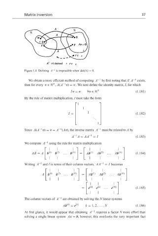
Figure 1.8 Defining A −1 is impossible when det(A) = 0.

We obtain a more efficient method of computing A −1 by first noting that if A −1 exists,
N
−1
then for every v ∈ , A(A v) = v . We next define the identity matrix, I, for which
Iv = v ∀v ∈ N (1.181)
By the rule of matrix multiplication, I must take the form
1
 
1
 
 
1
  (1.182)
I =  
 . . 
 . 
1
−1
−1
Since A(A v) = v = A (Av), the inverse matrix A −1 must be related to A by
A −1 A = AA −1 = I (1.183)
We compute A −1 using the rule for matrix multiplication
   
| | | | | |
b
AB = A  (1) b (2) ... b (N)  =  Ab (1) Ab (2) ... Ab (N)  (1.184)
| | | | | |
Writing A −1 and I in terms of their column vectors, AA −1 = I becomes
   
| | | | | |
A  ˜ a (1) ˜ a (2) ... a ˜ (N)  =  A˜a (1) A˜a (2) ... A˜a (N) 
| | | | | |
 
| | |
e
=  [1] e [2] ... e [N]  (1.185)
| | |
The column vectors of A −1 are obtained by solving the N linear systems

A˜a (k) = e [k] k = 1, 2,..., N (1.186)
At first glance, it would appear that obtaining A −1 requires a factor N more effort than
solving a single linear system Ax = b; however, this overlooks the very important fact