Page 111 - Numerical methods for chemical engineering

Bifurcation analysis 97

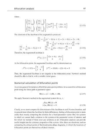
where
 ) *) * 

∂ f 1 ∂ f 1

 ∂x [k] ∂λ [k]  x [k] − f 1 (x,λ)


  = (2.153)
) *) * [k]

  λ − f 2 (x,λ)
 ∂ f 2 ∂ f 2 

∂x [k] ∂λ [k]
The elements of the Jacobian of the augmented system are
∂ f 1 ∂ 2
= {x + θ(λ)x + 1}= 2x + θ(λ) = 2x + 4λ
∂x ∂x
∂ f 1 ∂ 2 dθ
= {x + θ(λ)x + 1}= x = 4x
∂λ ∂λ dλ
∂ ∂ dθ
∂ f 2 ∂ f 2
= {2x + θ(λ)}= 2 = {2x + θ(λ)}= = 4 (2.154)
∂x ∂x ∂λ ∂λ dλ
Therefore, the augmented Jacobian is

(2x + 4λ)(4x)
(a)
J (x,λ) = (2.155)
2 4
At the bifurcation point, the augmented Jacobian and its determinant are

0 −4
(a)
J
J (−1, 0.5) = (a) = (0)(4) − (2)(−4) = 8 (2.156)
24
Thus, the augmented Jacobian is not singular at the bifurcation point. Newton’s method
should be able to find it, with a suitable initial guess.
Numerical calculation of bifurcation points
Asamoregeneralformulationofthebifurcationpointproblem,letussearchforabifurcation
point along the linear path in parameter space
(2.157)
Θ(λ) = (1 − λ)Θ 0 + λΘ 1
We apply Newton’s method to the augmented system for x s ,λ

f (x s ; Θ(λ)) = 0
|J(x s ; Θ(λ))| = 0 (2.158)
Clearly, as we must compute the determinant of the Jacobian at each Newton iteration, and
in general must obtain the Jacobian by finite differences, finding a bifurcation point is more
costly than merely computing the solution for a fixed parameter vector. But, for systems
in which we cannot find a solution to the system at the parameter vector of interest, and
for which we wonder if there exist any solutions at all, bifurcation analysis can provide
useful insight into the existence properties of the system. Also, there are situations, such as
computing the critical points of thermodynamic phase diagrams, in which the locations of
bifurcation points are themselves of direct interest.