Page 115 - Numerical methods for chemical engineering

Problems 101

c = H p A c = H p A
As
A
As
A
c (x)
A

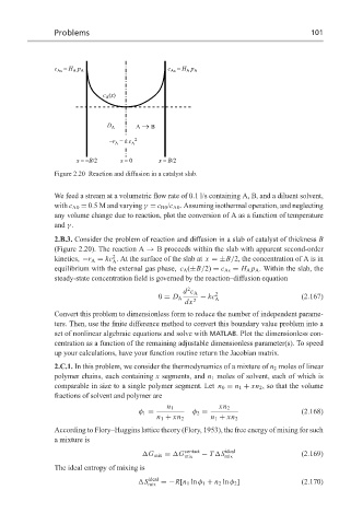
D A A → B

−r A = kc A 2
x = −B/2 x = 0 x = B/2
Figure 2.20 Reaction and diffusion in a catalyst slab.

We feed a stream at a volumetric flow rate of 0.1 l/s containing A, B, and a diluent solvent,
with c A0 = 0.5 M and varying γ = c B0 /c A0 . Assuming isothermal operation, and neglecting
any volume change due to reaction, plot the conversion of A as a function of temperature
and γ .
2.B.3. Consider the problem of reaction and diffusion in a slab of catalyst of thickness B
(Figure 2.20). The reaction A → B proceeds within the slab with apparent second-order
2
kinetics, −r A = kc . At the surface of the slab at x =±B/2, the concentration of A is in
A
equilibrium with the external gas phase, c A (±B/2) = c As = H A p A . Within the slab, the
steady-state concentration field is governed by the reaction–diffusion equation
2
d c A 2
0 = D A 2 − kc A (2.167)
dx
Convert this problem to dimensionless form to reduce the number of independent parame-
ters. Then, use the finite difference method to convert this boundary value problem into a
set of nonlinear algebraic equations and solve with MATLAB. Plot the dimensionless con-
centration as a function of the remaining adjustable dimensionless parameter(s). To speed
up your calculations, have your function routine return the Jacobian matrix.
2.C.1. In this problem, we consider the thermodynamics of a mixture of n 2 moles of linear
polymer chains, each containing x segments, and n 1 moles of solvent, each of which is
comparable in size to a single polymer segment. Let n 0 = n 1 + xn 2 , so that the volume
fractions of solvent and polymer are

n 1 xn 2
φ 1 = φ 2 = (2.168)
n 1 + xn 2 n 1 + xn 2
According to Flory–Huggins lattice theory (Flory, 1953), the free energy of mixing for such
a mixture is
G mix = G contact − T S ideal (2.169)
mix mix
The ideal entropy of mixing is

S ideal =−R[n 1 ln φ 1 + n 2 ln φ 2 ] (2.170)
mix