Page 120 - Numerical methods for chemical engineering

106 3 Matrix eigenvalue analysis

e u

u 2
α
e 2
e 1
α
u 1
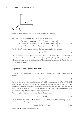
Figure 3.1 A counter-clockwise rotation in the 1–2 plane performed by Q.

To obtain the inverse rotation Q −1 , we obviously set α →−α,

   
cos(−α) − sin(−α)0 cos α sin α 0
Q −1 =  sin(−α) cos(−α) 0  =  − sin α cos α 0  = Q T (3.12)
0 0 1 0 0 1
For this Q, e [3] has the special property that it is unchanged by the rotation,

Qe [3] = e [3] (3.13)
[3]
Obviously, this is because Q defines a rotation about e . However, if we did not know this
but rather only knew the matrix elements of Q, recognizing that Qe [3] = e [3] immediately
tells us something useful about the nature of the transformation done by Q. This is the role
of eigenvalue analysis.

Eigenvalues and eigenvectors defined

If A is an N ×N matrix, and if w is acted upon by A simply as if it were multiplied by a
scalar λ,

Aw = λw (3.14)
then w is said to be a characteristic vector of A with the characteristic value λ. This field
was developed, to a large extent, by German mathematicians, and the German word for
characteristic value is “eigenwert,” eigen meaning characteristic, individual, or unique, and
wert meaning value or worth. It is now common, if confusing, practice to use the halb
Deutsch/half English terms eigenvalue and eigenvector.
As Iv = v, the “eigenpair” (w, λ) satisfies the linear system

(A − λI)w = 0 (3.15)
For this to hold true for w = 0, the matrix (A − λI) must be singular, providing a charac-
teristic polynomial of degree N,

p(λ) = det(A − λI) = 0 (3.16)
whose N roots are the eigenvalues of A.