Page 155 - Numerical methods for chemical engineering

Singular value decomposition (SVD) 141

1

12

1

eectrn densit

2

1 1 2

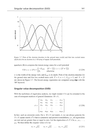
Figure 3.7 Plots of the electron densities in the ground state (solid) and first two excited states
(dash-dot) for an electron in a 1-D array of square well potentials.

quantum 1D.m computes the lowest energy states for a well potential
w w
−E well , P − 2 ≤ x ≤ P + 2
V (0 ≤ x ≤ 2P) = (3.229)
0, otherwise
w is the width of the energy well, and E well is its depth. Plots of the electron densities for
the ground state and first two excited states with P = 1, w = 1, E well = 5, and N = 25
are shown in Figure 3.7. The lowest energy eigenstates are computed using eigs with the
‘SR’ keyword.

Singular value decomposition (SVD)

With the usefulness of eigenvalue analysis, we might wonder if it can be extended to the
case of nonsquare matrices of general dimension M×N,

 
a 11 a 12 a 13 ... a 1N
 a 21 a 22 a 23 ... a 2N 
 
a 31 a 32 a 33 a 3N  (3.230)
 ... 
A = 
 . . .
 . . . . . . . 
.
. 
a M1 a M2 a M3 ... a MN
In fact, such an extension exists. For a M×N real matrix A, we can always generate the
T
N ×N square matrix A A that is symmetric and positive-semidefinite; i.e., all eigenvalues
T
are real and are greater than or equal to zero. Let the eigenvalues of A A be µ 1 , µ 2 ,...,
µ N . We then define the singular values of A as
√ √ √
σ 1 = µ 1 σ 2 = µ 2 ... σ N = µ N (3.231)