Page 157 - Numerical methods for chemical engineering

Singular value decomposition (SVD) 143

SVD analysis and the existence/uniqueness properties of linear systems

Let us examine how SVD aids detecting the existence and uniqueness properties of linear
systems. As noted in Chapter 1, the nature of the null space (kernel) of A and of the
range are vitally important; however, we have not described how we may identify these
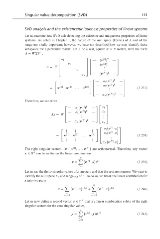
subspaces for a particular matrix. Let A be a real, square N × N matrix, with the SVD
T
A = W V ,
  [1] T
— (v ) —
σ 1  
σ 2 (v )
   — [2] T
  . — 
.  
A = W  .   . 
 .  .
—(v [N] T —
)
σ N
— σ 1 (v ) —
 [1] T 
 
| | | [2] T
 — σ 2 (v ) — 
=  w [1] w [2] ... w [N]   . .  (3.237)
 . 
| | | [N] T
— σ N (v ) —
Therefore, we can write
 
— σ 1 (v ) — x 1
 [1] T 
[2] T
 — σ 2 (v ) —   x 2 
Ax = W  . .   
.
 .   . 
 . 
)
— σ N (v [N] T —
x N
σ 1 v ·x
 [1] 
 
| | |  σ 2 v [2]

=  w [1] w [2] ... w [N]   . ·x  (3.238)

.
 
.
| | | [N]
σ N v ·x
[2]
[1]
The right singular vectors {v , v ,..., v [N] } are orthonormal. Therefore, any vector
N
x ∈ can be written as the linear combination
N

x = v [ j] · x v [ j] (3.239)
j=1
Let us say the first r singular values of A are zero and that the rest are nonzero. We want to
identify the null space K A and range R A of A. To do so, we break the linear contribution for
x into two parts
r N

x = v [ j] · x v [ j] + v [ j] · x v [ j] (3.240)
j=1 j=r+1
σ j =0 σ j >0
N
Let us now define a second vector y ∈ that is a linear combination solely of the right
singular vectors for the zero singular values,
r

y = v [ j] · y v [ j] (3.241)
j=1
σ j =0