Page 162 - Numerical methods for chemical engineering

148 3 Matrix eigenvalue analysis

S inv =
0.1578 0 0 0 0
0 0.7981 0 0 0
0 0 0.8878 0 0
*
*
*

b=V S inv U y,
b=
1.0000
2.0000
3.0000
Thus, the fitted parameters of the linear model are β 0 = 1,β 1 = 2,β 2 = 3. This approach
to the design and analysis of data sets for parameter estimation will be considered again in
Chapter 8.

Computing the roots of a polynomial

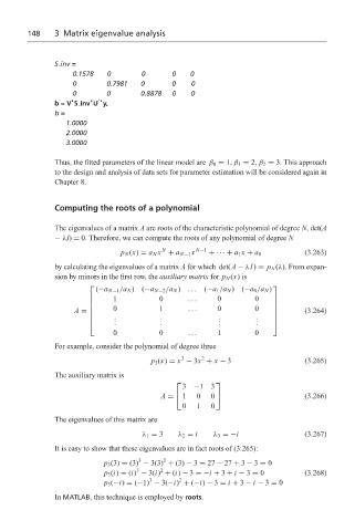
The eigenvalues of a matrix A are roots of the characteristic polynomial of degree N, det(A
− λI) = 0. Therefore, we can compute the roots of any polynomial of degree N
N
p N (x) = a N x + a N−1 x N−1 + ··· + a 1 x + a 0 (3.263)
by calculating the eigenvalues of a matrix A for which det(A − λI) = p N (λ). From expan-
sion by minors in the first row, the auxiliary matrix for p N (x)is
(−a N−1 /a N )(−a N−2 /a N ) ... (−a 1 /a N )(−a 0 /a N )
 
1 0 ... 0 0
 
 
 0 1 ... 0 0 
A =   (3.264)
. . . .
. . . .
 
 . . . . 
0 0 ... 1 0
For example, consider the polynomial of degree three
2
3
p 3 (x) = x − 3x + x − 3 (3.265)
The auxiliary matrix is
3 −13
 
A =  1 0 0  (3.266)
0 1 0
The eigenvalues of this matrix are

λ 1 = 3 λ 2 = i λ 3 =−i (3.267)
It is easy to show that these eigenvalues are in fact roots of (3.265):
2
3
p 3 (3) = (3) − 3(3) + (3) − 3 = 27 − 27 + 3 − 3 = 0
3
2
p 3 (i) = (i) − 3(i) + (i) − 3 =−i + 3 + i − 3 = 0 (3.268)
3
2
p 3 (−i) = (−1) − 3(−i) + (−i) − 3 = i + 3 − i − 3 = 0
In MATLAB, this technique is employed by roots.