Page 164 - Numerical methods for chemical engineering

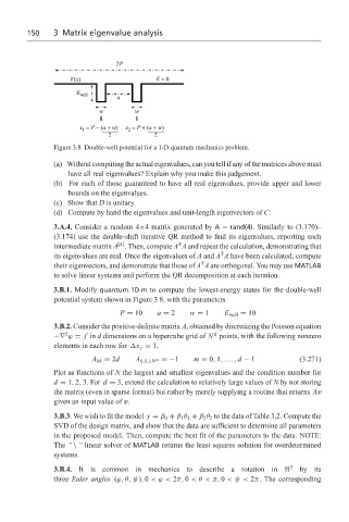
150 3 Matrix eigenvalue analysis

2P

V(x) E = 0
E well
a
w w

x = P − (a + w) x = P + (a + w)
2
1
2 2
Figure 3.8 Double-well potential for a 1-D quantum mechanics problem.
(a) Without computing the actual eigenvalues, can you tell if any of the matrices above must
have all real eigenvalues? Explain why you make this judgement.
(b) For each of those guaranteed to have all real eigenvalues, provide upper and lower
bounds on the eigenvalues.
(c) Show that D is unitary.
(d) Compute by hand the eigenvalues and unit-length eigenvectors of C.

3.A.4. Consider a random 4×4 matrix generated by A = rand(4). Similarly to (3.170)–
(3.174) use the double-shift iterative QR method to find its eigenvalues, reporting each
T
[k]
intermediate matrix A . Then, compute A A and repeat the calculation, demonstrating that
T
its eigenvalues are real. Once the eigenvalues of A and A A have been calculated, compute
T
their eigenvectors, and demonstrate that those of A A are orthogonal. You may use MATLAB
to solve linear systems and perform the QR decomposition at each iteration.
3.B.1. Modify quantum 1D.m to compute the lowest-energy states for the double-well
potential system shown in Figure 3.8, with the parameters
P = 10 a = 2 w = 1 E well = 10
3.B.2. Consider the positive-definite matrix A, obtained by discretizing the Poisson equation
d
2
−∇ ϕ = f in d dimensions on a hypercube grid of N points, with the following nonzero
elements in each row for x j = 1,
A kk = 2d A k,k±N =−1 m = 0, 1,..., d − 1 (3.271)
m
Plot as functions of N the largest and smallest eigenvalues and the condition number for
d = 1, 2, 3. For d = 3, extend the calculation to relatively large values of N by not storing
the matrix (even in sparse format) but rather by merely supplying a routine that returns Av
given an input value of v.
3.B.3. We wish to fit the model y = β 0 + β 1 θ 1 + β 2 θ 2 to the data of Table 3.2. Compute the
SVD of the design matrix, and show that the data are sufficient to determine all parameters
in the proposed model. Then, compute the best fit of the parameters to the data. NOTE:
The “ \ ” linear solver of MATLAB returns the least squares solution for overdetermined
systems.
3
3.B.4. It is common in mechanics to describe a rotation in by its
three Euler angles (ϕ, θ, ψ), 0 <ϕ < 2π, 0 <θ <π, 0 <ψ < 2π. The corresponding