Page 161 - Numerical methods for chemical engineering

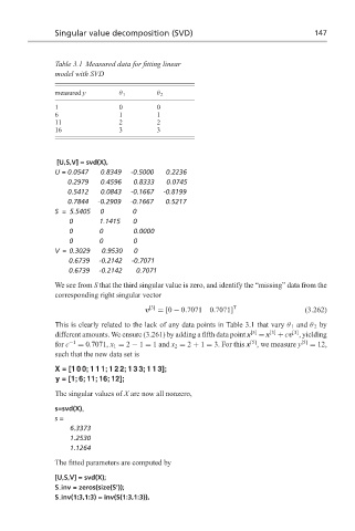
Singular value decomposition (SVD) 147

Table 3.1 Measured data for fitting linear
model with SVD

measured y θ 1 θ 2
1 0 0
6 1 1
11 2 2
16 3 3

[U,S,V] = svd(X),
U = 0.0547 0.8349 -0.5000 0.2236
0.2979 0.4596 0.8333 0.0745
0.5412 0.0843 -0.1667 -0.8199
0.7844 -0.2909 -0.1667 0.5217
S = 5.5405 0 0
0 1.1415 0
0 0 0.0000
0 0 0
V = 0.3029 0.9530 0
0.6739 -0.2142 -0.7071
0.6739 -0.2142 0.7071
We see from S that the third singular value is zero, and identify the “missing” data from the
corresponding right singular vector
v [3] = [0 − 0.7071 0.7071] T (3.262)

This is clearly related to the lack of any data points in Table 3.1 that vary θ 1 and θ 2 by
[3]
different amounts. We ensure (3.261) by adding a fifth data point x [5] = x [3] + cv , yielding
[5]
for c −1 = 0.7071, x 1 = 2 − 1 = 1 and x 2 = 2 + 1 = 3. For this x , we measure y [5] = 12,
such that the new data set is
X = [100;111;122;133;113];
y = [1; 6; 11; 16; 12];
The singular values of X are now all nonzero,

s=svd(X),
s=
6.3373
1.2530
1.1264

The fitted parameters are computed by
[U,S,V] = svd(X);
S inv = zeros(size(S’));
S inv(1:3,1:3) = inv(S(1:3,1:3)),