Page 163 - Numerical methods for chemical engineering

Problems 149

MATLAB summary

The use of MATLAB to compute eigenvalues was discussed earlier in this chapter; therefore,
here only a brief summary is provided. A matrix W, whose column vectors are eigenvec-
tors of A, and a diagonal matrix D, whose principal diagonal contains the corresponding
eigenvalues, are returned by

[W,D] = eig(A);

Withonlyasingleoutputargument, eigreturnsavectorofeigenvalues.Ifonlyafewextremal
eigenvalues are desired, use eigs. For example, the five largest-magnitude eigenvalues of A
and the corresponding eigenvectors are returned by

[W,D] = eigs(A,5, ‘LM’);
Other options include computing the smallest magnitude (‘SM’), largest and smallest real
part (‘LR’, ‘SR’), or the eigenvalues closest to a specified target shift value. Type help eigs,
or consult the earlier discussion of this chapter, for further details.
H
The SVD A = USV is computed by
[U,S,V] = svd(A);

The condition number is computed by cond and condest; the norm by norm and normest;
and the rank by rank. Eigenvalue methods are used to compute all roots of a polynomial by
roots.

Problems

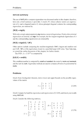
3.A.1. From Gershgorin’s theorem, derive lower and upper bounds on the possible eigen-
values of the matrix
10 3
 
A =  02 1  (3.269)
31 −1

3.A.2. Compute by hand the eigenvalues and eigenvectors of (3.269), and check your results
using MATLAB.
3.A.3. Consider the following matrices,
0 −1 −2 1  
 
6 2 1
−1 2 0 4
 
A =   B =  0 5 −1 
−2 0 3 0
 
−13 2
1 4 0 −1
(3.270)
0 −10
 

3 2
C = D =  1 0 0 
1 −1
0 0 1