Page 183 - Numerical methods for chemical engineering

Linear ODE systems and dynamic stability 169

Thus, as f s ≈ f exact , we have the approximate value for the integral
' 1 ' 1
f (x, y) r≤1 (x, y)dxdy ≈ A sd f s
−1 −1
N s
A sd $ [k] [k] % $ [k] [k] %
= f x , y r≤1 x , y (4.88)
N s
k=1
The following code uses this method to obtain an approximate value for the integral of
(4.82) in good agreement with that obtained from dblquad.
Numlter = 5000000; % increase for greater accuracy
f sum=0;
for iter = 1:Numlter
*
x = -1 + 2*rand; y = -1 + 2 rand;
r=xˆ2+yˆ2;
if(r <=1)
* *
*
f sum=f sum+xˆ2+2 yˆ2-2 x y;
end
end
f avg=f sum/Numlter;
area = 4;
*
int 2D MC = f avg area,
int 2D MC = 2.3563

Linear ODE systems and dynamic stability

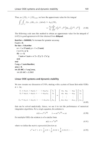
We now resume our discussion of IVPs, starting with a system of linear first-order ODEs
˙ x = Ax,
     
˙ x 1 = a 11 x 1 + a 12 x 2 +· · · + a 1N x N ˙ x 1 a 11 a 12 ··· a 1N x 1
˙ x 2 = a 21 x 1 + a 22 x 2 +· · · + a 2N x N  ˙ x 2   a 21 a 22 ··· a 2N   x 2 
     
.  .  =  . . .   . 
. . . .
.
.  .   . . .   . 
.
˙ x N = a N1 x 1 + a N2 x 2 +· · · + a NN x N ˙ x N a N1 a N2 ··· a NN x N
(4.89)
that can be solved analytically. Hence, we use it to test the performance of numerical
integration algorithms. For a single equation, the solution is
at [0]
at [0]
x(t) = e x ˙ x = ae x = ax (4.90)
For multiple ODEs the solution is of a similar form
At [0]
x(t) = e x (4.91)
where we define the matrix exponential function as
1 1 1
A
e = I + A + AA + AAA + AAAA +· · · (4.92)
2! 3! 4!