Page 188 - Numerical methods for chemical engineering

174 4 Initial value problems

12
11
t 1
1

1 1 2
t
11
1
t
2
1

1 1 2
t
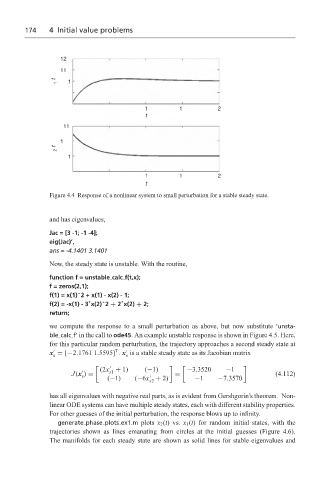
Figure 4.4 Response of a nonlinear system to small perturbation for a stable steady state.

and has eigenvalues,
Jac = [3 -1; -1 -4];
eig(Jac)’,
ans = -4.1401 3.1401

Now, the steady state is unstable. With the routine,
function f = unstable calc f(t,x);
f = zeros(2,1);
f(1) = x(1)ˆ2+x(1)-x(2)-1;
*
*
f(2) = -x(1) - 3 x(2)ˆ2 + 2 x(2) + 2;
return;
we compute the response to a small perturbation as above, but now substitute ‘unsta-
ble calc f’ in the call to ode45. An example unstable response is shown in Figure 4.5. Here,
for this particular random perturbation, the trajectory approaches a second steady state at
T

x = [−2.1761 1.5595] . x is a stable steady state as its Jacobian matrix
s
s

(2x + 1) (−1) −3.3520 −1

s1
J(x ) = = (4.112)
s
(−1) (−6x + 2) −1 −7.3570
s2
has all eigenvalues with negative real parts, as is evident from Gershgorin’s theorem. Non-
linear ODE systems can have multiple steady states, each with different stability properties.
For other guesses of the initial perturbation, the response blows up to infinity.
generate phase plots ex1.m plots x 2 (t) vs. x 1 (t) for random initial states, with the
trajectories shown as lines emanating from circles at the initial guesses (Figure 4.6).
The manifolds for each steady state are shown as solid lines for stable eigenvalues and