Page 193 - Numerical methods for chemical engineering

Overview of ODE-IVP solvers in MATLAB 179

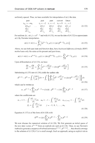
uniformly spaced. Thus, we have available for interpolation of x(τ) the data
past past past current future
=−m h τ 2 =−2 τ 1 =−1 τ 0 = 0 τ −1 = 1
τ m h
) ... x(τ 2 ) x(τ 1 ) x(τ 0 ) x(τ −1 ) (4.132)

x(τ m h
dx dx dx dx dx

dτ dτ dτ dτ dτ
τ m h τ τ τ τ −1
2 1 0
For uniform t, x(τ j ) = x [k− j] and with (4.131), we use the data of (4.132) to approximate
x(τ) by Hermite interpolation,
m h

x(τ) ≈ π(τ) = x [k− j] L j0 (τ) + ( t) f [k− j] L j1 (τ) (4.133)
j=−1
Above, we use both past state and function data, but a backward difference formula (BDF)
method uses only the states at the present and past times,
m h
[k− j]
[k+1]
[k+1]
x(τ) ≈ π(τ) = x L −1,0 (τ) + ( t) f L −1,1 (τ) + x L j0 (τ) (4.134)
j=0
Upon differentiation of (4.133), we have
m h
dx dπ [k− j] dL j0 [k− j] dL j1
≈ = x + ( t) f (4.135)
dτ dτ dτ dτ
j=−1
Substituting (4.135) into (4.130) yields the update rule
(
m h
' 1 dπ ' 1 dL j0 dL j1
x [k+1] − x [k] = dτ = x [k− j] + ( t) f [k− j] dτ
0 dt 0 j=−1 dτ dτ
(4.136)
which can be written as
m h m h
[k− j] [k+1] [k− j]
[k+1]
α −1 x + α j x = ( t)β −1 f + ( t) β j f (4.137)
j=0 j=0
where the coefficients are
' 1 ' 1 ' 1
dL −1,0 dL 00 dL j0
α −1 = 1 − dτ α 0 =−1 − dτ α j∈ [1,m h ] =− dτ
0 dτ 0 dτ 0 dτ
1
'
dL j1
β j = dτ j =−1, 0, 1, ..., m h
0 dτ
(4.138)
Equation (4.137) is of the form of (4.128) with
m h m h
[k] [k− j] [k− j]
U = ( t) β j f − α j x (4.139)
j=0 j=1
We now discuss the numerical solution of (4.128). We first generate an initial guess of
the new state vector, x [k+1,0] from an explicit rule such as (4.118). Then, we use Newton’s
method to generate a sequence of refined estimates x [k+1,1] , x [k+1,2] , . . . that should converge
to the solution of (4.128) if t is small enough. Such an approach, using an explicit rule to