Page 192 - Numerical methods for chemical engineering

178 4 Initial value problems

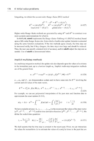
Integrating, we obtain the second-order Runge–Kutta (RK2) method

3
x [k+1] − x [k] = k (2) + O( t )
(1)

k (1) = ( t) f x [k] k (2) = ( t) f x [k] + k /2 (4.127)
2
3
local error ∼ O( t ) global error ∼ O( t )
Higher-order Runge–Kutta methods are generated by using k (1) and k (2) to construct even
more accurate approximations for f (x(t)).
In MATLAB, ode45 implements the Runge–Kutta–Fehlberg 4-5 (RKF45) method, based
upon a fifth-order Runge–Kutta rule, from which a fourth-order update formula is extracted
using the same function evaluations. If the two methods agree closely, the time step can
be increased safely, but if they disagree, the time step is too large and should be reduced.
Thus, the user can specify a desired level of accuracy, and let ode45 adjust the step size as
needed. Use of ode45 is demonstrated below.

Implicit multistep methods

In a multistep integration method, the update rule also depends upon the values of x at times
in the immediate past, up to a horizon length m h . Implicit multi-step integration methods
are of the general form

α −1 x [k+1] + α 0 x [k] = ( t)β −1 f x [k+1] ; Θ + U [k] (4.128)
α −1 ,α 0 , and β −1 are dimensionless scalars and we have some rule for U [k] involving the
current and old values of the state vector,

[k] [k] [k−1] [k−2] [k−m h ]
U = F t, f (x; Θ); t k , x , t k−1 , x , t k−2 , x , ..., t k−m h , x
(4.129)
For example, we can use polynomial interpolation of the past state and function data to
approximate the exact update (4.114),

' t k + t ' 1 dx
x(t k + t) − x [k] = f (x(t))dt = dτ τ ≡ t − t k (4.130)
0 dτ t
t k
}intherecentpastthevaluesofthestatevector
Wehaveavailableattimes {t k , t k−1 ,..., t k−m h
[k]
{x , x [k−1] ,..., x [k−m h ] } and the time derivative function { f [k] , f [k−1] ,..., f [k−m h ] }.We
define the scaled time quantities

t k− j − t k dx dt dx [k− j]
τ j = ˙ x(τ j ) = = = ( t) f x (4.131)
t dτ dτ dt
x [k− j] x [k− j]
We shall assume that the time step is constant in the recent past. If not, we can interpolate
the values for nonuniform t to estimate the values of x and f at times in the past that are