Page 185 - Numerical methods for chemical engineering

Linear ODE systems and dynamic stability 171

w
Aw λ w
e (λ

initia initia w s
state state
stead state stae anid
initia Aw λ w s
s
state s
e (λ
s
initia
state nstae anid

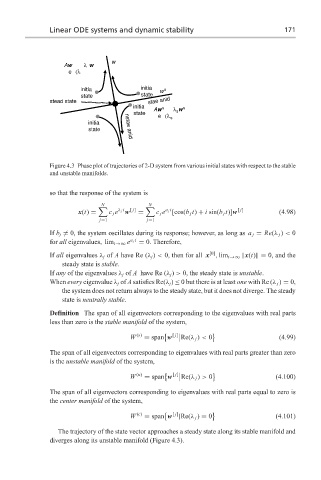
Figure 4.3 Phase plot of trajectories of 2-D system from various initial states with respect to the stable
and unstable manifolds.

so that the response of the system is
N N
λ j t [ j] a j t [ j]
x(t) = c j e w = c j e [cos(b j t) + i sin(b j t)]w (4.98)
j=1 j=1
If b j = 0, the system oscillates during its response; however, as long as a j = Re(λ j ) < 0
for all eigenvalues, lim t→∞ e a j t = 0. Therefore,
[0]
If all eigenvalues λ j of A have Re (λ j ) < 0, then for all x , lim t→∞ x(t) = 0, and the
steady state is stable.
If any of the eigenvalues λ j of A have Re (λ j ) > 0, the steady state is unstable.
When every eigenvalue λ j of A satisfies Re(λ j ) ≤ 0 but there is at least one with Re (λ j ) = 0,
the system does not return always to the steady state, but it does not diverge. The steady
state is neutrally stable.
Definition The span of all eigenvectors corresponding to the eigenvalues with real parts
less than zero is the stable manifold of the system,

W (s) = span w [ j] Re(λ j ) < 0 (4.99)
The span of all eigenvectors corresponding to eigenvalues with real parts greater than zero
is the unstable manifold of the system,

W (u) = span w [ j] Re(λ j ) > 0 (4.100)
The span of all eigenvectors corresponding to eigenvalues with real parts equal to zero is
the center manifold of the system,

[ j]

W (c) = span w |Re(λ j ) = 0 (4.101)
The trajectory of the state vector approaches a steady state along its stable manifold and
diverges along its unstable manifold (Figure 4.3).