Page 33 - Numerical methods for chemical engineering

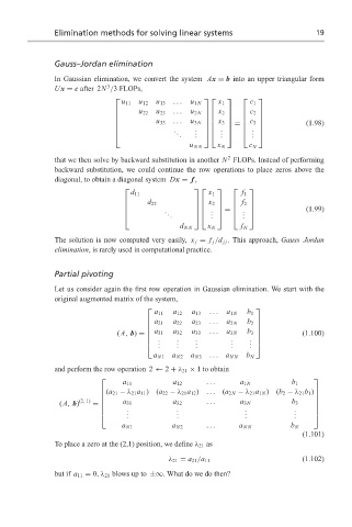
Elimination methods for solving linear systems 19

Gauss–Jordan elimination

In Gaussian elimination, we convert the system Ax = b into an upper triangular form
3
Ux = c after 2N /3 FLOPs,
     
u 11 u 12 u 13 ... u 1N x 1 c 1
 u 22 u 23 ... u 2N   x 2   c 2 
     
u 33 (1.98)
 ...     
 u 3N   x 3  =  c 3 
.
 . .   .   . 
.
.
 . . .   .   . 
u NN x N c N
2
that we then solve by backward substitution in another N FLOPs. Instead of performing
backward substitution, we could continue the row operations to place zeros above the
diagonal, to obtain a diagonal system Dx = f ,
     
d 11 x 1 f 1
 d 22   x 2   f 2 
      (1.99)
.
 .   .  =  . 
.
.
 .   .   . 
d NN x N f N
The solution is now computed very easily, x j = f j /d jj . This approach, Gauss–Jordan
elimination, is rarely used in computational practice.
Partial pivoting
Let us consider again the first row operation in Gaussian elimination. We start with the
original augmented matrix of the system,
 
a 11 a 12 a 13 ... a 1N b 1
 a 21 ... 
a 22 a 23 a 2N b 2
 
 ... 
a 31 a 32 a 33 a 3N (1.100)
(A, b) =  b 3 
 . . . .
 . . . . . . . . . 
.
. 
a N1 a N2 a N3 ... a NN b N
and perform the row operation 2 ← 2 + λ 21 × 1 to obtain
 
a 11 a 12 ... a 1N b 1
 (a 21 − λ 21 a 11 )(a 22 − λ 21 a 12 )
... (a 2N − λ 21 a 1N )(b 2 − λ 21 b 1 ) 
 
(A, b) (2, 1) =  a 31 a 32 ... a 3N b 3 


. . . .
. . . .
 
 . . . . 
...
a N1 a N2 a NN b N
(1.101)
To place a zero at the (2,1) position, we define λ 21 as
(1.102)
λ 21 = a 21 /a 11
but if a 11 = 0,λ 21 blowsupto ±∞. What do we do then?