Page 118 - Optofluidics Fundamentals, Devices, and Applications

Optofluidic Trapping and Transport Using Planar Photonic Devices 99

needed to release a particle compared to the random thermal motion
of the particle, which is important on such size ranges [16]:

W F γ −1
S = trap = T0 f 1 [ + θ(ln( θ) − 1)] (5-15)
kT kT
B B
where S = stability number
k = Boltzmann number
B
T = temperature of the system.
S can take values greater than or equal to zero, with zero repre-
senting a critically unstable trap.
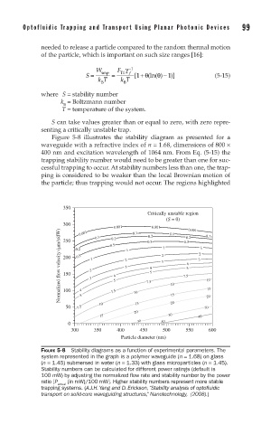
Figure 5-8 illustrates the stability diagram as presented for a
waveguide with a refractive index of n = 1.68, dimensions of 800 ×
400 nm and excitation wavelength of 1064 nm. From Eq. (5-15) the
trapping stability number would need to be greater than one for suc-
cessful trapping to occur. At stability numbers less than one, the trap-
ping is considered to be weaker than the local Brownian motion of
the particle; thus trapping would not occur. The regions highlighted

350
Critically unstable region
(S = 0)
300 0.001 0.1 0.2 0.001 0.1 0.5 0.001 0.1 0.5 0.2 0.001 0.1
Normalized flow velocity (μm/s/dW) 200 0.2 3 2 1 0.5 4 5 2 3 1 7.5 4 5 2 3 1 10 7.5 4 5 3 2 1 10
0.2
250
0.5

150

100
20
20
50 7.5 4 5 10 7.5 10 15 15 30 15
20
15 30 40
30 40
0
300 350 400 450 500 550 600
Particle diameter (nm)
FIGURE 5-8 Stability diagrams as a function of experimental parameters. The
system represented in the graph is a polymer waveguide (n = 1.68) on glass
(n = 1.45) submersed in water (n = 1.33) with glass microparticles (n = 1.45).
Stability numbers can be calculated for different power ratings (default is
100 mW) by adjusting the normalized fl ow rate and stability number by the power
ratio [P (in mW)/100 mW]. Higher stability numbers represent more stable
actual
trapping systems. (A.J.H. Yang and D. Erickson, “Stability analysis of optofl uidic
transport on solid-core waveguiding structures,” Nanotechnology, (2008).)