Page 70 - Origin and Prediction of Abnormal Formation Pressures

52 G.V. CHILINGAR, J.O. ROBERTSON JR. AND H.H. RIEKE III
1.0
1.0
0.9
0.8
0.8
0.7
0.6
0.6
t~ 0.5

4:: 0.4
0.4
0.3
0.2
0.2
z/i :0.1

01111
I 0 4 10 .3 I 0 "2 10 I I I 0
Kt/Ss 12

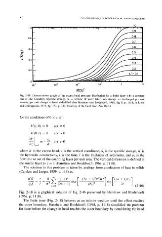
Fig. 2-18. Dimensionless graph of the excess-head pressure distribution for a finite layer with a constant
flux at one boundary. Specific storage, Ss = volume of water taken into storage, or discharged per unit
volume, per unit change in head. (Modified after Hanshaw and Bredehoeft, 1968, fig. 9, p. 1118; in Rieke
and Chilingarian, 1974, fig. 177, p. 331. Courtesy of the Geol. Soc. Am. Bull.)

for the conditions of 0 < z < 1

h'(z, 0) - 0 att - 0
h'(O, t) - 0 att > 0

ah' qo
= att >0
0z z=t K
where h' is the excess head, z is the vertical coordinate, S~ is the specific storage, K is
the hydraulic conductivity, t is the time, l is the thickness of sediments, and qo is the
flow into or out of the confining layer per unit area. The vertical dimension is defined at
the source layer as z -- 1 (Hanshaw and Bredehoeft, 1968, p. 1118).
The solution to this problem is taken by analogy from conduction of heat in solids
(Carslaw and Jaeger, 1959, p. 113) as"
h'K_z 8 L (-1) n [-(2n+l)27r2Kt] [(2n + 1)7rz]
qol -- 1 7/-2 ,,=0 (2n + 1----~ exp 4S~12 sin 21 (2-46)

Fig. 2-18 is a graphical solution of Eq. 2-46 presented by Hanshaw and Bredehoeft
(1968, p. 1118).
The finite zone (Fig. 2-18) behaves as an infinite medium until the effect reaches
the outer boundary. Hanshaw and Bredehoeft (1968, p. 1118) simplified the problem
for time before the change in head reaches the outer boundary by considering the head