Page 72 - Origin and Prediction of Abnormal Formation Pressures

54 G.V. CHILINGAR, J.O. ROBERTSON JR. AND H.H. RIEKE III
-1
10

10 .2

o
O"
E:
10 .3

lo-4t

-7 l I I i I li:
10 10 .6 10 .5 10 .4 10 .3 10 .2
ktlSs 12

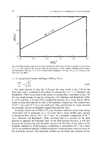
Fig. 2-20. Dimensionless graph of excess-head variation for small values of time at a surface of constant flux
(z/1 = 1). The solution is the same for either the semi-infinite or finite medium. (Modified after Hanshaw
and Bredehoeft, 1968, fig. I1, p. 1119; in Rieke and Chilingarian, 1974, fig. 179, p. 332. Courtesy of the
Geol. Soc. Am. Bull.)

z = 0, was given by Carslaw and Jaeger (1959, p. 75) as:

h'K = 2/Kt
(2-49)
qo V Jr S~
For small intervals of time, Eq. 2-49 gives the same results as Eq. 2-45 for the
finite layer that is evaluated at the surface of constant flux (z/l = 1) (Hanshaw and
Bredehoeft, 1968). Excess head at the surface of constant flux is presented in Fig. 2-20
for very small amounts of time by solving Eq. 2-45. Hanshaw and Bredehoeft (1968,
p. 1119) used Figs. 2-19 and 2-20 to compute the pressure, for a source bed at 1200 m
depth, overlain and underlain by beds of low hydraulic conductivity. The conductivities
of 10 -12 cm/s and 10 -l~ cm/s were both used. They reported that the results obtained
are extremely sensitive to hydraulic conductivities and flow rates.
Assuming a burial rate of 500 m/106 years, the phase transition period (time during
which fluid will be produced) for a 15-m-thick bed is about 30,000 years; upward
or downward flow will be 3.85 x 10 -~~ cm/s. At a hydraulic conductivity of 10 -12
cm/s, Hanshaw and Bredehoeft (1968) calculated that it is possible for the fluid
pressure to approach the lithostatic load. As the fluid pressure increases, it will also
decrease the reaction rate and, therefore, decrease the fluid flux at low values of the
hydraulic conductivity. If the hydraulic conductivity is increased to 10 -1~ cm/s, there
will be an insufficient quantity of fluid produced to create pressures much in excess of
the hydrostatic pressure. The important variables are the burial rate, thickness of the