Page 383 - Petrophysics 2E

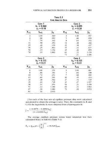
VERTICAL SATURATION PROFILE IN A RESERVOIR 351

TABLE 5.3
CORE ANALYSIS DATA
Core 1 Core 2
kl = 0.060 k2 = 0.095
= 0.18 01 = 0.20

Pclj Swlj Jlj pc2j Sw2j J2j
3 1 .oo .Ob9 3 1 .oo .057
4 .88 ,092 5 .80 .095
7 .70 .162 8 .64 ,152
11 .58 .254 14 .48 .266
19 .40 .439 23 .38 .437
36 .25 .832 33 .32 .627
56 .19 1.294 45 .26 355
78 .19 1.802 61 .22 1.159
74 .21 1.406
Core 3 Core 4
k3 = 0.132 = 0.155
03 = 0.21 @4 = 0.23

Pc3j Sw3j J3j Pc4j sw4j J4j
6 1 .oo .151 3 1 .oo .051
8 .86 ,201 4 .84 .108
10 .72 .251 7 .68 .189
12 .60 .301 16 .45 .432
20 .48 .502 27 .34 .729
29 .40 .728 41 .27 1.107
38 .34 ,954 54 .21 1.458
51 .32 1.280 69 .21 1.863
67 .30 1.682 76 .20 2.052
81 .30 2.033

J for each of the four sets of capillary pressure data were calculated
and plotted to obtain the average J-curve. Then, the constants (A, B, and
C) for the hyperbolic fit were obtained from a least-squares fit.

(-0.0075 - 0.2856 Swj)
j=
(1 + 0.0391 Swj)

The average capillary pressure versus water saturation was then
calculated from J as follows (Table 5.4):