Page 221 - Phase Space Optics Fundamentals and Applications

202 Chapter Six

(a) (b)

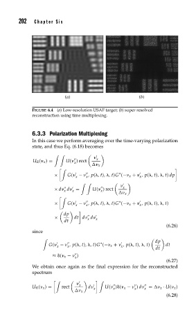
FIGURE 6.4 (a) Low-resolution USAF target; (b) super resolved
reconstruction using time multiplexing.

6.3.3 Polarization Multiplexing
In this case we perform averaging over the time-varying polarization
state, and thus Eq. (6.18) becomes

x

U R ( x ) = U( ) rect
x
x

∗

× G( − ,p( ,t), ,t)G (− x + ,p( ,t), ,t) dp
x
x
x

x
× d d = U( ) rect
x
x
x
x

∗

× G( − ,p( ,t), ,t)G (− x + ,p( ,t), ,t)
x x x

dp

× dt d d x
x
dt
(6.26)
since

dp
G( − ,p( ,t), ,t)G (− x + ,p( ,t), ,t) dt

∗

x
x
x
dt
≈ ( x − )

x
(6.27)
We obtain once again as the final expression for the reconstructed
spectrum

x

U R ( x ) = rect d x U( ) ( x − ) d = x · U( x )
x
x
x
x
(6.28)