Page 224 - Phase Space Optics Fundamentals and Applications

Super Resolved Imaging in Wigner-Based Phase Space 205

(a) (b)

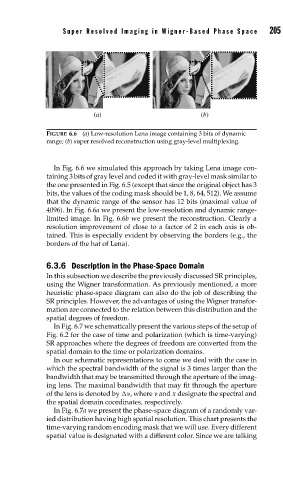
FIGURE 6.6 (a) Low-resolution Lena image containing 3 bits of dynamic
range; (b) super resolved reconstruction using gray-level multiplexing.

In Fig. 6.6 we simulated this approach by taking Lena image con-
taining 3 bits of gray level and coded it with gray-level mask similar to
the one presented in Fig. 6.5 (except that since the original object has 3
bits, the values of the coding mask should be 1, 8, 64, 512). We assume
that the dynamic range of the sensor has 12 bits (maximal value of
4096). In Fig. 6.6a we present the low-resolution and dynamic range-
limited image. In Fig. 6.6b we present the reconstruction. Clearly a
resolution improvement of close to a factor of 2 in each axis is ob-
tained. This is especially evident by observing the borders (e.g., the
borders of the hat of Lena).

6.3.6 Description in the Phase-Space Domain
In this subsection we describe the previously discussed SR principles,
using the Wigner transformation. As previously mentioned, a more
heuristic phase-space diagram can also do the job of describing the
SR principles. However, the advantages of using the Wigner transfor-
mation are connected to the relation between this distribution and the
spatial degrees of freedom.
In Fig. 6.7 we schematically present the various steps of the setup of
Fig. 6.2 for the case of time and polarization (which is time-varying)
SR approaches where the degrees of freedom are converted from the
spatial domain to the time or polarization domains.
In our schematic representations to come we deal with the case in
which the spectral bandwidth of the signal is 3 times larger than the
bandwidth that may be transmitted through the aperture of the imag-
ing lens. The maximal bandwidth that may fit through the aperture
of the lens is denoted by , where and x designate the spectral and
the spatial domain coordinates, respectively.
In Fig. 6.7a we present the phase-space diagram of a randomly var-
ied distribution having high spatial resolution. This chart presents the
time-varying random encoding mask that we will use. Every different
spatial value is designated with a different color. Since we are talking