Page 227 - Phase Space Optics Fundamentals and Applications

208 Chapter Six

ν ν

3Δν x Δν x

λ, dynamic range λ, dynamic range
(a) (b)
ν

Δν x

λ
(c)

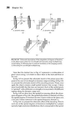
FIGURE 6.8 Schematic description of the adaptation of degrees of freedom
in the phase-space plane for wavelength and dynamic range multiplexing.
(a) Encoding. (b) Blurring due to reduced resolution of the imaging system.
(c) Decoding for wavelength multiplexing.

Note that the dashed line in Fig. 6.7 represents a continuation of
pixel values along x of which we show three at the start and three at
the end.
In Fig. 6.8 we present the schematic sketch of the phase-space dia-
gram in the case of wavelength or dynamic range encoding. In Fig. 6.8a
we present the schematic sketch of the encoding process. There, once
again the object contains small spatial features that occupy 3 times
more bandwidth that the lens can transmit. Each of the spatial pixels
is “painted” with a different wavelength or is associated with different
regions along the dynamic range axis.
In Fig. 6.8b we show how the spatial low passing affects the phase-
space diagram of Fig. 6.8a. The spatial information is blurred, and thus
the spatial degrees of freedom become 3 times wider in the space axis
x but also 3 times narrower in the spatial-frequency domain x .
In Fig. 6.8c we present the schematic effect of the decoding. Here in
each one of the spatial degrees of freedom is multiplied by a proper
spatially high-resolution distribution which corresponds to the spatial