Page 337 - Phase Space Optics Fundamentals and Applications

318 Chapter Ten

10.2.5 The Comb Function and Rect Function
10.2.5.1 Comb Functions
In sampling theory one cannot avoid encountering both comb func-
tions and rect functions. For example, the physical sampling of a signal
is modeled by multiplying by a train of Dirac delta functions, some-
times called a comb function T (x),
∞ ∞
, 1 , j2 nx
T (x) = (x − nT) = exp (10.12)
T T
n=−∞ n=−∞
where the rightmost part of Eq. (10.12) comes from a Fourier series
expansion. The WDF of this comb function can be expressed as 47

∞ ∞
1 , , n + m ! n − m "
{ T (x)}(x, k) = k − exp j2 x
T 2 2T T
n=−∞ m=−∞
(10.13)
Equation (10.13) can be expanded out into the following form:
∞ ∞
1 , , nm n mT
{ T (x)}(x, k) = (−1) k − x −
2T 2T 2
n=−∞ m=−∞
(10.14)
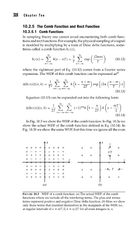
In Fig. 10.3 we show the WDF of the comb function. In Fig. 10.3a we
show the actual WDF of the comb function defined in Eq. (10.14). In
Fig. 10.3b we show the same WDF, but this time we ignore all the even

k k

1/T
x x

T

(a) (b)

FIGURE 10.3 WDF of a comb function. (a) The actual WDF of the comb
functions where we include all the interfering terms. The plus and minus
terms represent positive and negative Dirac delta function. (b) Here we show
only those terms that manifest themselves in the marginals of the WDF, i.e.,
at regular intervals of x = mT/2,k = n/2T for all even integers m, n.