Page 181 - Physical Principles of Sedimentary Basin Analysis

6.15 Cooling sills and dikes 163

g(x)
1.0

0.5
f(x)
f(x), g(x) 0.0

−0.5

−1.0
−6 −4 −2 0 2 4 6
x
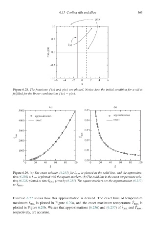
Figure 6.28. The functions f (x) and g(x) are plotted. Notice how the initial condition for a sill is
fulfilled for the linear combination f (x) − g(x).

(a) (b)
5000 0.05
approximation approximation
4000 exact 0.04 exact

3000 0.03
^ max t ^ T max
2000 0.02

1000 0.01

0 0.00
0 20 40 60 80 100 0 20 40 60 80 100
^ z z ^

Figure 6.29. (a) The exact solution (6.235)for ˆ t max is plotted as the solid line, and the approxima-
tion (6.236)to ˆ t max is plotted with the square markers. (b) The solid line is the exact temperature solu-
tion (6.228) plotted at time ˆ t max given by (6.235). The square markers are the approximation (6.237)
to ˆ T max .

Exercise 6.27 shows how this approximation is derived. The exact time of temperature
ˆ
maximum ˆ t max is plotted in Figure 6.29a, and the exact maximum temperature T max is
ˆ
plotted in Figure 6.29b. We see that approximations (6.236) and (6.237)of ˆ t max and T max ,
respectively, are accurate.