Page 396 - Power Electronic Control in Electrical Systems

//SYS21/F:/PEC/REVISES_10-11-01/075065126-CH009.3D ± 375 ± [373±406/34] 17.11.2001 10:33AM

Power electronic control in electrical systems 375

9.2 A basic worked example ± leading and lagging loads

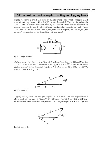
Figure 9.1 shows a circuit with a supply system whose open-circuit voltage is E and
short-circuit impedance is Z s ˆ 0 ‡ jX s , where X s ˆ 0:1
. The load impedance is
Z ˆ 1
but the power factor can be unity, 0.8 lagging, or 0.8 leading. For each of
these three cases, the supply voltage E must be adjusted to keep the terminal voltage
V ˆ 100 V. For each case determine E, the power-factor angle f, the load angle d, the
power P, the reactive power Q, and the volt-amperes S.

Fig. 9.1 Simple AC circuit.

Unity power-factor. Referring to Figure 9.2, we have E cos d ˆ V ˆ 100 and E sin d ˆ
X s I ˆ 0:1 100/1 ˆ 10 V. Therefore E ˆ 100 ‡ j10 ˆ 100:5e j5:71 V. The power-factor
j0
angleisf ˆ cos 1 (1) ˆ 0,d ˆ 5:71 ,andS ˆ P ‡ jQ ˆ VI ˆ 100 100e ˆ 10 kVA,

with P ˆ 10 kW and Q ˆ 0.

Fig. 9.2 Unity PF.

Lagging power-factor. Referring to Figure 9.3, the current is rotated negatively to a
phase angle of f ˆ cos 1 (0:8) ˆ 36:87 . Although I ˆ 100 A and X s I is still 10 V,

its new orientation `stretches'the phasor E to a larger magnitude: E ˆ V ‡ jX s I ˆ

Fig. 9.3 Lagging PF.