Page 51 - Practical Control Engineering a Guide for Engineers, Managers, and Practitioners

26 Chapter Two

1.2
1
::s
.& 0.8
g 0.6
~ 0.4
e 0.2
Q..
0
0 10 20 30 40 50 60 70 80 90 100

1
&_o.s
.5 0.6
(/)
] ~:~

0-
0 10 20 30 40 50 60 70 80 90 100
Time (sec)

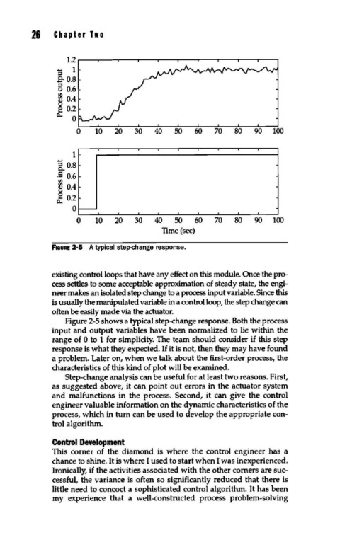
fiGURE 2·5 A typical step-change response.

existing control loops that have any effect on this module. Once the pr<r
cess settles to some acceptable approximation of steady state, the engi-
neer makes an isolated step change to a process input variable. Since this
is usually the manipulated variable in a control loop, the step change can
often be easily made via the actuator.
Figure 2-5 shows a typical step-change response. Both the process
input and output variables have been normalized to lie within the
range of 0 to 1 for simplicity. The team should consider if this step
response is what they expected. If it is not, then they may have found
a problem. Later on, when we talk about the first-order process, the
characteristics of this kind of plot will be examined.
Step-change analysis can be useful for at least two reasons. First,
as suggested above, it can point out errors in the actuator system
and malfunctions in the process. Second, it can give the control
engineer valuable information on the dynamic characteristics of the
process, which in turn can be used to develop the appropriate con-
trol algorithm.
Control Development
This corner of the diamond is where the control engineer has a
chance to shine. It is where I used to start when I was inexperienced.
Ironically, if the activities associated with the other corners are suc-
cessful, the variance is often so significantly reduced that there is
little need to concoct a sophisticated control algorithm. It has been
my experience that a well-constructed process problem-solving