Page 84 - Practical Control Engineering a Guide for Engineers, Managers, and Practitioners

Basic Concepts in Process Analysis 59

simplest is to break the expression for Y into simple algebraic terms and
then go to the mentioned box of Laplace transforms and find the corre-
sponding time domain function. We will get into this soon but, first, a
few comments about the transfer function G,in Eq. (3-33).

3-3-1 The Transfer Function and Block Diagram Algebra
The introduction of the transfer function GP(s) in Eq. (3-33) is useful
because of the block diagram interpretation (Fig. 3-9). The expression
in the box multiplies the input to the box to give the box's output.
Alternatively, one can play some games with Eq.(3-33) and get

Y=-g-ii
'l'S+1
- - -
Y+-rsY=gU
(3-34)
-rsY=gii- Y

-
-)
1(1)( -
Y=-; ~ gU-Y
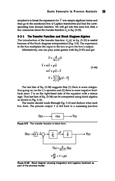
The last line of Eq. (3-34) suggests that (1) there is some integra-
tion going o~ via the 1 Is operator and (2) there is some negative feed-
back since Y is on the right-hand side of the equation with a minus
sign. That last line of Eq. (3-34) can be interpreted using block algebra
as shown in Fig. 3-10.
The reader should wade through Fig. 3-10 and deduce what each
box does. The process output Y is fed back to a summing junction

U(s) Y(s)

FIGURE 3-9 The transfer function in block form.

O(s)~~--·
Y(s)
-~

Y(s) =_L_ D(s)
ts+ 1
t~; + Y=gU

FIGURE 3-10 Block diagram showing integration and negative feedback as
part of the process model.