Page 97 - Practical Control Engineering a Guide for Engineers, Managers, and Practitioners

72 Chapter Three

The term pole" may come from the appearance of the magni-
11
tude of a Laplace transform when plotted in the s-domain. Consider
the first-order Laplace transform

s)=-g ___ 3_
G(
-rs+1- s+3
g = 1 'f = 0.3333
which has a pole at s = -3. The magnitude of G(s) can be obtained
from its complex conjugate, as explained in App. F, as

s=a+ jb
3 3
G(s) = -r(a + jb) + 3 -ra + 3 + j-rb

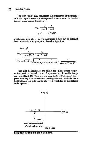
First, plot the location of the pole in the s-plane where a repre-
sents a point on the real axis and b represents a point on the imagi-
nary axis (Fig. 3-13). Next, plot the magnitude of G(s) against the s-
plane as in Fig. 3-14. Notice how the magnitude of G(s) looks like a
tent that has a tent pole located at s = -3.0 which lies on the real axis
in the s-plane.

Imag(s)

-1/t=-3.0
------iT---+----- Real (s)

First-order model has
a ''real" pole p here
1
Thes-plane
F1eURE 3-13 Location of a pole in the s-plane.