Page 162 - Principles of Applied Reservoir Simulation 2E

Part II: Reservoir Simulation 147

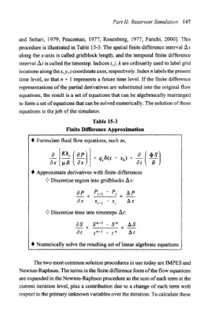
and Settari, 1979; Peaceman, 1977; Rosenberg, 1977; Fanchi, 2000]. This
procedure is illustrated in Table 15-3. The spatial finite difference interval AJC
along the jc-axis is called gridblock length, and the temporal finite difference
interval Ads called the timestep. Indices ij, k are ordinarily used to label grid
locations along the*,;;, z coordinate axes, respectively. Index n labels the present
time level, so that n + 1 represents a future time level. If the finite difference
representations of the partial derivatives are substituted into the original flow
equations, the result is a set of equations that can be algebraically rearranged
to form a set of equations that can be solved numerically. The solution of these
equations is the job of the simulator.

Table 15-3
Finite Difference Approximation
Formulate fluid flow equations, such as,

Kk a

dx 8*1 B
Approximate derivatives with finite differences
0 Discretize region into gridblocks AJC:

dx x. +l - jc. AJC

0 Discretize time into timesteps A/:
n 1
BS S * - S n _
dt t n + l - t n Af

Numerically solve the resulting set of linear algebraic equations

The two most common solution procedures in use today are IMPES and
Newton-Raphson. The terms in the finite difference form of the flow equations
are expanded in the Newton-Raphson procedure as the sum of each term at the
current iteration level, plus a contribution due to a change of each term with
respect to the primary unknown variables over the iteration. To calculate these