Page 164 - Principles of Applied Reservoir Simulation 2E

Part II: Reservoir Simulation 149

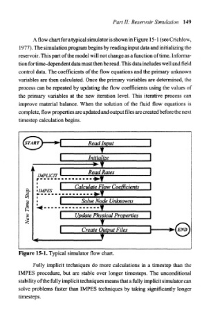
A flow chart for a typical simulator is shown in Figure 15-1 (see Crichlow,
1977). The simulation program begins by reading input data and initializing the
reservoir. This part of the model will not change as a function of time. Informa-
tion for time-dependent data must then be read. This data includes well and field
control data. The coefficients of the flow equations and the primary unknown
variables are then calculated. Once the primary variables are determined, the
process can be repeated by updating the flow coefficients using the values of
the primary variables at the new iteration level. This iterative process can
improve material balance. When the solution of the fluid flow equations is
complete, flow properties are updated and output files are created before the next
timestep calculation begins.

Read Input

Initialize
±3.
I Read Rates I
IMPLICIT
r
Coefficients
I M Calculate Flow M M I
MM
g IMPES ^™ ™*™**™^ ^*^*^y** ^^ **^^'^'*^*'
50 I Solve Node Unknowns \
s
\ Update Physical Properties \
v
I Create Output Files

Figure 15-1. Typical simulator flow chart.

Fully implicit techniques do more calculations in a timestep than the
IMPES procedure, but are stable over longer timesteps. The unconditional
stability of the fully implicit techniques means that a fully implicit simulator can
solve problems faster than IMPES techniques by taking significantly longer
timesteps.